ValidMind for development 3 — Integrate custom tests

Learn how to use ValidMind for your end-to-end documentation process with our series of four introductory notebooks. In this third notebook, supplement ValidMind tests with your own and include them as additional evidence in your documentation.

This notebook assumes that you already have a repository of custom made tests considered critical to include in your documentation. A custom test is any function that takes a set of inputs and parameters as arguments and returns one or more outputs:

• The function can be as simple or as complex as you need it to be — it can use external libraries, make API calls, or do anything else that you can do in Python.
• The only requirement is that the function signature and return values can be "understood" and handled by the ValidMind Library. As such, custom tests offer added flexibility by extending the default tests provided by ValidMind, enabling you to document any type of record (model) or use case.

For a more in-depth introduction to custom tests, refer to our Implement custom tests notebook.

Learn by doing

Our course tailor-made for developers new to ValidMind combines this series of notebooks with more a more in-depth introduction to the ValidMind Platform — Developer Fundamentals

Prerequisites

In order to integrate custom tests with your documentation with this notebook, you'll need to first have:

• Registered a model within the ValidMind Platform with a predefined documentation template
• Installed the ValidMind Library in your local environment, allowing you to access all its features
• Learned how to import and initialize datasets for use with ValidMind
• Understood the basics of how to run and log tests with ValidMind
• Inserted a test-driven block for the results of your HighPearsonCorrelation:balanced_raw_dataset test into your model's documentation

Need help with the above steps?

Refer to the first two notebooks in this series:

• 1 — Set up the ValidMind Library
• 2 — Start the development process

Setting up

This section should be quite familiar to you — as we performed the same actions in the previous notebook, 2 — Start the development process.

Initialize the ValidMind Library

As usual, let's first connect up the ValidMind Library to our model we previously registered in the ValidMind Platform:

1. On the left sidebar that appears for your model, select Getting Started and select Development from the Document drop-down menu.

2. Click Copy snippet to clipboard.

3. Next, load your model identifier credentials from an .env file or replace the placeholder with your own code snippet:

# Make sure the ValidMind Library is installed

%pip install -q validmind

# Load your model identifier credentials from an `.env` file

%load_ext dotenv
%dotenv .env

# Or replace with your code snippet

import validmind as vm

vm.init(
    # api_host="...",
    # api_key="...",
    # api_secret="...",
    # model="...",
    document="documentation",
)

Note: you may need to restart the kernel to use updated packages.

2026-09-11 23:48:18,490 - INFO(validmind.api_client): 🎉 Connected to ValidMind!
📊 Model: [ValidMind Academy] Model development (ID: cmalgf3qi02ce199qm3rdkl46)
📁 Document Type: model_documentation

Import sample dataset

Next, we'll import the same public Bank Customer Churn Prediction dataset from Kaggle we used in the last notebook so that we have something to work with:

from validmind.datasets.classification import customer_churn as demo_dataset

print(
    f"Loaded demo dataset with: \n\n\t• Target column: '{demo_dataset.target_column}' \n\t• Class labels: {demo_dataset.class_labels}"
)

raw_df = demo_dataset.load_data()

Loaded demo dataset with: 

    • Target column: 'Exited' 
    • Class labels: {'0': 'Did not exit', '1': 'Exited'}

We'll apply a simple rebalancing technique to the dataset before continuing:

import pandas as pd

raw_copy_df = raw_df.sample(frac=1)  # Create a copy of the raw dataset

# Create a balanced dataset with the same number of exited and not exited customers
exited_df = raw_copy_df.loc[raw_copy_df["Exited"] == 1]
not_exited_df = raw_copy_df.loc[raw_copy_df["Exited"] == 0].sample(n=exited_df.shape[0])

balanced_raw_df = pd.concat([exited_df, not_exited_df])
balanced_raw_df = balanced_raw_df.sample(frac=1, random_state=42)

Remove highly correlated features

Let's also quickly remove highly correlated features from the dataset using the output from a ValidMind test.

As you learned previously, before we can run tests you'll need to initialize a ValidMind dataset object:

# Register new data and now 'balanced_raw_dataset' is the new dataset object of interest
vm_balanced_raw_dataset = vm.init_dataset(
    dataset=balanced_raw_df,
    input_id="balanced_raw_dataset",
    target_column="Exited",
)

With our balanced dataset initialized, we can then run our test and utilize the output to help us identify the features we want to remove:

# Run HighPearsonCorrelation test with our balanced dataset as input and return a result object
corr_result = vm.tests.run_test(
    test_id="validmind.data_validation.HighPearsonCorrelation",
    params={"max_threshold": 0.3},
    inputs={"dataset": vm_balanced_raw_dataset},
)

❌ High Pearson Correlation

The High Pearson Correlation test evaluates pairwise linear relationships among dataset features to identify highly correlated pairs that may indicate redundancy or multicollinearity. The result table reports the top feature pairs ranked by Pearson correlation coefficient and classifies each pair against the configured absolute correlation threshold of 0.3. Across the 10 reported pairs, coefficients range from -0.1892 to 0.3543, with one pair exceeding the threshold and the remaining pairs classified as passing.

Key insights:

• One pair exceeds threshold: The pair (Age, Exited) has the largest reported correlation, with a coefficient of 0.3543, and is the only pair marked Fail against the 0.3 threshold.
• Remaining correlations are low in magnitude: The other nine reported feature pairs have absolute correlation values below 0.19, and all are marked Pass.
• Observed relationships are mostly weak: Outside the top result, the largest absolute coefficients are -0.1892 for (IsActiveMember, Exited) and -0.1875 for (Balance, NumOfProducts), followed by 0.1590 for (Balance, Exited).
• Both positive and negative associations appear: The reported coefficients include positive values such as (Age, Balance) = 0.0570 and negative values such as (Tenure, IsActiveMember) = -0.0420, indicating mixed linear relationship directions across the listed pairs.

The reported correlation structure is concentrated in a single threshold breach, with (Age, Exited) standing apart from the rest of the listed relationships. All other reported pairwise correlations remain below the configured cutoff and are modest in absolute magnitude. Overall, the table shows limited high linear dependence among the top reported feature pairs, with one identified exception.

Parameters:

{
  "max_threshold": 0.3
}
            

Tables

Columns	Coefficient	Pass/Fail
(Age, Exited)	0.3543	Fail
(IsActiveMember, Exited)	-0.1892	Pass
(Balance, NumOfProducts)	-0.1875	Pass
(Balance, Exited)	0.1590	Pass
(NumOfProducts, Exited)	-0.0639	Pass
(Age, Balance)	0.0570	Pass
(Age, NumOfProducts)	-0.0518	Pass
(Tenure, IsActiveMember)	-0.0420	Pass
(Tenure, Exited)	-0.0388	Pass
(NumOfProducts, IsActiveMember)	0.0364	Pass

# From result object, extract table from `corr_result.tables`
features_df = corr_result.tables[0].data
features_df

	Columns	Coefficient	Pass/Fail
0	(Age, Exited)	0.3543	Fail
1	(IsActiveMember, Exited)	-0.1892	Pass
2	(Balance, NumOfProducts)	-0.1875	Pass
3	(Balance, Exited)	0.1590	Pass
4	(NumOfProducts, Exited)	-0.0639	Pass
5	(Age, Balance)	0.0570	Pass
6	(Age, NumOfProducts)	-0.0518	Pass
7	(Tenure, IsActiveMember)	-0.0420	Pass
8	(Tenure, Exited)	-0.0388	Pass
9	(NumOfProducts, IsActiveMember)	0.0364	Pass

# Extract list of features that failed the test
high_correlation_features = features_df[features_df["Pass/Fail"] == "Fail"]["Columns"].tolist()
high_correlation_features

['(Age, Exited)']

# Extract feature names from the list of strings
high_correlation_features = [feature.split(",")[0].strip("()") for feature in high_correlation_features]
high_correlation_features

['Age']

We can then re-initialize the dataset with a different input_id and the highly correlated features removed and re-run the test for confirmation:

# Remove the highly correlated features from the dataset
balanced_raw_no_age_df = balanced_raw_df.drop(columns=high_correlation_features)

# Re-initialize the dataset object
vm_raw_dataset_preprocessed = vm.init_dataset(
    dataset=balanced_raw_no_age_df,
    input_id="raw_dataset_preprocessed",
    target_column="Exited",
)

# Re-run the test with the reduced feature set
corr_result = vm.tests.run_test(
    test_id="validmind.data_validation.HighPearsonCorrelation",
    params={"max_threshold": 0.3},
    inputs={"dataset": vm_raw_dataset_preprocessed},
)

✅ High Pearson Correlation

The High Pearson Correlation test evaluates pairwise linear relationships among features to identify potentially redundant variables or multicollinearity. The result table reports the top 10 feature pairs ranked by Pearson correlation coefficient using a maximum threshold of 0.3 for pass/fail assessment. The reported coefficients range from -0.1892 to 0.1590, and each listed pair is marked as Pass. The strongest observed relationships in the output are between IsActiveMember and Exited, Balance and NumOfProducts, and Balance and Exited.

Key insights:

• No pair exceeds threshold: All reported feature pairs pass the test against the 0.3 threshold. The largest absolute coefficient in the output is 0.1892, which remains below the configured limit.
• Observed relationships are weak: The top-ranked correlations are limited in magnitude, with the strongest negative correlation at -0.1892 for IsActiveMember and Exited and the strongest positive correlation at 0.1590 for Balance and Exited.
• Top correlations are concentrated in a few variables: Balance, Exited, IsActiveMember, NumOfProducts, and Tenure appear repeatedly across the top 10 reported pairs, while the associated coefficients remain small in absolute value.
• Both positive and negative associations are present: The output includes negative coefficients such as -0.1892, -0.1875, and -0.0639, as well as positive coefficients such as 0.1590, 0.0364, and 0.0359, indicating mixed directional relationships among the listed pairs.

The reported correlation structure indicates that none of the top 10 pairwise linear relationships breaches the configured threshold for high correlation. The strongest observed associations are weak in absolute magnitude, and all listed pairs are classified as Pass. Based on the reported output, the test does not identify highly correlated feature pairs among the top-ranked relationships shown.

Parameters:

{
  "max_threshold": 0.3
}
            

Tables

Columns	Coefficient	Pass/Fail
(IsActiveMember, Exited)	-0.1892	Pass
(Balance, NumOfProducts)	-0.1875	Pass
(Balance, Exited)	0.1590	Pass
(NumOfProducts, Exited)	-0.0639	Pass
(Tenure, IsActiveMember)	-0.0420	Pass
(Tenure, Exited)	-0.0388	Pass
(NumOfProducts, IsActiveMember)	0.0364	Pass
(Tenure, EstimatedSalary)	0.0359	Pass
(HasCrCard, Exited)	-0.0334	Pass
(CreditScore, EstimatedSalary)	-0.0305	Pass

Train the model

We'll then use ValidMind tests to train a simple logistic regression model on our prepared dataset:

# First encode the categorical features in our dataset with the highly correlated features removed
balanced_raw_no_age_df = pd.get_dummies(
    balanced_raw_no_age_df, columns=["Geography", "Gender"], drop_first=True
)
balanced_raw_no_age_df.head()

	CreditScore	Tenure	Balance	NumOfProducts	HasCrCard	IsActiveMember	EstimatedSalary	Exited	Geography_Germany	Geography_Spain	Gender_Male
318	593	4	129499.42	1	1	1	154071.27	0	True	False	False
5171	687	6	0.00	2	0	0	179206.92	0	False	False	False
480	699	4	0.00	2	0	1	111307.98	0	False	False	True
4719	588	9	67178.19	1	1	1	163534.75	1	False	True	False
2575	580	0	125647.36	1	1	0	57541.08	1	False	False	True

# Split the processed dataset into train and test
from sklearn.model_selection import train_test_split

train_df, test_df = train_test_split(balanced_raw_no_age_df, test_size=0.20)

X_train = train_df.drop("Exited", axis=1)
y_train = train_df["Exited"]
X_test = test_df.drop("Exited", axis=1)
y_test = test_df["Exited"]

from sklearn.linear_model import LogisticRegression

# Logistic Regression grid params
log_reg_params = {
    "penalty": ["l1", "l2"],
    "C": [0.001, 0.01, 0.1, 1, 10, 100, 1000],
    "solver": ["liblinear"],
}

# Grid search for Logistic Regression
from sklearn.model_selection import GridSearchCV

grid_log_reg = GridSearchCV(LogisticRegression(), log_reg_params)
grid_log_reg.fit(X_train, y_train)

# Logistic Regression best estimator
log_reg = grid_log_reg.best_estimator_

Initialize the ValidMind objects

Let's initialize the ValidMind Dataset and Model objects in preparation for assigning predictions to each dataset:

# Initialize the datasets into their own ValidMind dataset objects
vm_train_ds = vm.init_dataset(
    input_id="train_dataset_final",
    dataset=train_df,
    target_column="Exited",
)

vm_test_ds = vm.init_dataset(
    input_id="test_dataset_final",
    dataset=test_df,
    target_column="Exited",
)

# Initialize the ValidMind model object
vm_model = vm.init_model(log_reg, input_id="log_reg_model_v1")

Assign predictions

Once the model is registered, we'll assign predictions to the training and test datasets:

vm_train_ds.assign_predictions(model=vm_model)
vm_test_ds.assign_predictions(model=vm_model)

2026-09-11 23:48:28,436 - INFO(validmind.vm_models.dataset.utils): Running predict_proba()... This may take a while
2026-09-11 23:48:28,437 - INFO(validmind.vm_models.dataset.utils): Done running predict_proba()
2026-09-11 23:48:28,438 - INFO(validmind.vm_models.dataset.utils): Running predict()... This may take a while
2026-09-11 23:48:28,439 - INFO(validmind.vm_models.dataset.utils): Done running predict()
2026-09-11 23:48:28,442 - INFO(validmind.vm_models.dataset.utils): Running predict_proba()... This may take a while
2026-09-11 23:48:28,444 - INFO(validmind.vm_models.dataset.utils): Done running predict_proba()
2026-09-11 23:48:28,445 - INFO(validmind.vm_models.dataset.utils): Running predict()... This may take a while
2026-09-11 23:48:28,446 - INFO(validmind.vm_models.dataset.utils): Done running predict()

Implementing a custom inline test

With the set up out of the way, let's implement a custom inline test that calculates the confusion matrix for a binary classification model.

• An inline test refers to a test written and executed within the same environment as the code being tested — in this case, right in this Jupyter Notebook — without requiring a separate test file or framework.
• You'll note that the custom test function is just a regular Python function that can include and require any Python library as you see fit.

Create a confusion matrix plot

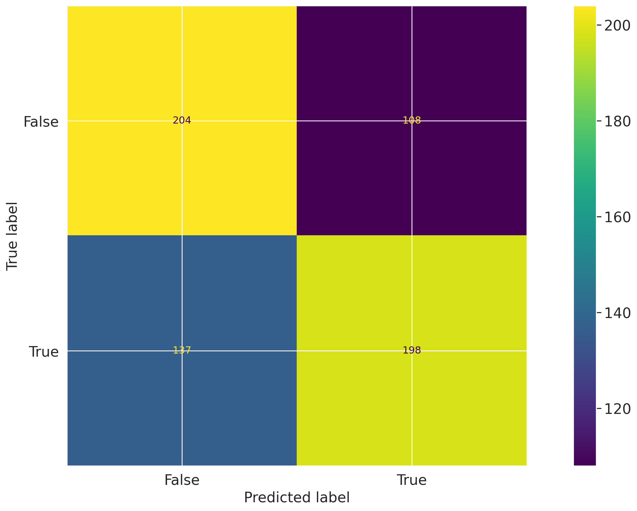
Let's first create a confusion matrix plot using the confusion_matrix function from the sklearn.metrics module:

import matplotlib.pyplot as plt
from sklearn import metrics

# Get the predicted classes
y_pred = log_reg.predict(vm_test_ds.x)

confusion_matrix = metrics.confusion_matrix(y_test, y_pred)

cm_display = metrics.ConfusionMatrixDisplay(
    confusion_matrix=confusion_matrix, display_labels=[False, True]
)
cm_display.plot()

Next, create a @vm.test wrapper that will allow you to create a reusable test. Note the following changes in the code below:

• The function confusion_matrix takes two arguments dataset and model. This is a VMDataset and VMModel object respectively.
  • VMDataset objects allow you to access the dataset's true (target) values by accessing the .y attribute.
  • VMDataset objects allow you to access the predictions for a given record (model) by accessing the .y_pred() method.
• The function docstring provides a description of what the test does. This will be displayed along with the result in this notebook as well as in the ValidMind Platform.
• The function body calculates the confusion matrix using the sklearn.metrics.confusion_matrix function as we just did above.
• The function then returns the ConfusionMatrixDisplay.figure_ object — this is important as the ValidMind Library expects the output of the custom test to be a plot or a table.
• The @vm.test decorator is doing the work of creating a wrapper around the function that will allow it to be run by the ValidMind Library. It also registers the test so it can be found by the ID my_custom_tests.ConfusionMatrix.

@vm.test("my_custom_tests.ConfusionMatrix")
def confusion_matrix(dataset, model):
    """The confusion matrix is a table that is often used to describe the performance of a classification model on a set of data for which the true values are known.

    The confusion matrix is a 2x2 table that contains 4 values:

    - True Positive (TP): the number of correct positive predictions
    - True Negative (TN): the number of correct negative predictions
    - False Positive (FP): the number of incorrect positive predictions
    - False Negative (FN): the number of incorrect negative predictions

    The confusion matrix can be used to assess the holistic performance of a classification model by showing the accuracy, precision, recall, and F1 score of the model on a single figure.
    """
    y_true = dataset.y
    y_pred = dataset.y_pred(model=model)

    confusion_matrix = metrics.confusion_matrix(y_true, y_pred)

    cm_display = metrics.ConfusionMatrixDisplay(
        confusion_matrix=confusion_matrix, display_labels=[False, True]
    )
    cm_display.plot()

    plt.close()  # close the plot to avoid displaying it

    return cm_display.figure_  # return the figure object itself

You can now run the newly created custom test on both the training and test datasets using the run_test() function:

# Training dataset
result = vm.tests.run_test(
    "my_custom_tests.ConfusionMatrix:training_dataset",
    inputs={"model": vm_model, "dataset": vm_train_ds},
)

Confusion Matrix Training Dataset

The Confusion Matrix test evaluates classification performance by comparing predicted labels with true labels on the training dataset. The matrix reports counts for true negatives, false positives, false negatives, and true positives across the two outcome classes. In this result, the four cells contain 858 true negatives, 457 false positives, 479 false negatives, and 791 true positives, providing a direct view of correct and incorrect classifications by class.

Key insights:

• Correct classifications exceed errors: The model records 858 true negatives and 791 true positives, compared with 457 false positives and 479 false negatives. Both classes therefore contain more correct than incorrect classifications on the training dataset.

• Negative class is identified more accurately: True negatives total 858, while true positives total 791. This indicates a higher count of correct classifications for the negative class than for the positive class.

• Error counts are relatively balanced: False positives and false negatives are close in magnitude, at 457 and 479 respectively. This indicates that misclassification is distributed across both error types rather than concentrated in one direction.

The training confusion matrix shows that the model correctly classifies both negative and positive cases more often than it misclassifies them. Correct negative classifications are slightly higher than correct positive classifications, while false positives and false negatives are similar in count. Overall, the result reflects a relatively balanced classification pattern across classes with comparable error levels on both sides.

Figures

# Test dataset
result = vm.tests.run_test(
    "my_custom_tests.ConfusionMatrix:test_dataset",
    inputs={"model": vm_model, "dataset": vm_test_ds},
)

Confusion Matrix Test Dataset

The ConfusionMatrix:test_dataset test evaluates classification outcomes by comparing predicted labels against true labels in a 2x2 confusion matrix. The displayed matrix shows counts for true negatives, false positives, false negatives, and true positives on the test dataset. Observed cell values are 206 for true negatives, 95 for false positives, 139 for false negatives, and 207 for true positives.

Key insights:

• Correct predictions are balanced across classes: The model records 206 true negatives and 207 true positives, indicating nearly equal counts of correct classifications for the negative and positive classes.
• False negatives exceed false positives: The matrix shows 139 false negatives versus 95 false positives, indicating more missed positive cases than incorrect positive predictions.
• Positive class detection is mixed: While 207 positive cases are correctly identified, 139 positive cases are classified as negative, showing that correct positive detection is accompanied by a substantial number of missed positives.
• Negative class predictions are comparatively stronger: For the negative class, 206 cases are correctly classified compared with 95 cases misclassified as positive, yielding fewer errors than observed for the positive class.

The confusion matrix indicates that the model produces substantial correct classification counts in both classes, with true negatives and true positives at nearly identical levels. The main asymmetry in the error profile is the higher number of false negatives relative to false positives. Overall, the test results show balanced correct classifications across classes with a comparatively larger share of missed positive cases.

Figures

Add parameters to custom tests

Custom tests can take parameters just like any other function. To demonstrate, let's modify the confusion_matrix function to take an additional parameter normalize that will allow you to normalize the confusion matrix:

@vm.test("my_custom_tests.ConfusionMatrix")
def confusion_matrix(dataset, model, normalize=False):
    """The confusion matrix is a table that is often used to describe the performance of a classification model on a set of data for which the true values are known.

    The confusion matrix is a 2x2 table that contains 4 values:

    - True Positive (TP): the number of correct positive predictions
    - True Negative (TN): the number of correct negative predictions
    - False Positive (FP): the number of incorrect positive predictions
    - False Negative (FN): the number of incorrect negative predictions

    The confusion matrix can be used to assess the holistic performance of a classification model by showing the accuracy, precision, recall, and F1 score of the model on a single figure.
    """
    y_true = dataset.y
    y_pred = dataset.y_pred(model=model)

    if normalize:
        confusion_matrix = metrics.confusion_matrix(y_true, y_pred, normalize="all")
    else:
        confusion_matrix = metrics.confusion_matrix(y_true, y_pred)

    cm_display = metrics.ConfusionMatrixDisplay(
        confusion_matrix=confusion_matrix, display_labels=[False, True]
    )
    cm_display.plot()

    plt.close()  # close the plot to avoid displaying it

    return cm_display.figure_  # return the figure object itself

Pass parameters to custom tests

You can pass parameters to custom tests by providing a dictionary of parameters to the run_test() function.

• The parameters will override any default parameters set in the custom test definition. Note that dataset and model are still passed as inputs.
• Since these are VMDataset or VMModel inputs, they have a special meaning.
• When declaring a dataset, model, datasets or models argument in a custom test function, the ValidMind Library will expect these get passed as inputs to run_test() or run_documentation_tests().

Re-running the confusion matrix with normalize=True and our testing dataset looks like this:

# Test dataset with normalize=True
result = vm.tests.run_test(
    "my_custom_tests.ConfusionMatrix:test_dataset_normalized",
    inputs={"model": vm_model, "dataset": vm_test_ds},
    params={"normalize": True}
)

Confusion Matrix Test Dataset Normalized

The ConfusionMatrix test evaluates classification outcomes by comparing predicted labels to true labels, and this result presents the normalized confusion matrix for the test dataset. The matrix shows the proportion of observations in each true/predicted label combination rather than raw counts. The four displayed cells are 0.32 for true negatives, 0.15 for false positives, 0.21 for false negatives, and 0.32 for true positives.

Key insights:

• Correct classifications are evenly split: The normalized true negative and true positive cells are both 0.32, indicating equal proportions of correct predictions for the negative and positive classes in the displayed matrix.
• False negatives exceed false positives: The false negative cell is 0.21, while the false positive cell is 0.15. This shows a higher share of actual positive cases classified as negative than actual negative cases classified as positive.
• Diagonal cells dominate off-diagonal cells: The two correct-classification cells sum to 0.64, compared with 0.36 across the two error cells. This indicates that correct predictions account for a larger share of outcomes than misclassifications in the normalized result.

The normalized confusion matrix shows that correct predictions make up the majority of outcomes, with equal contribution from true negatives and true positives. Misclassification is present in both directions, with a larger proportion of false negatives than false positives. Overall, the result reflects balanced correct classification across classes alongside an asymmetry in error distribution.

Parameters:

{
  "normalize": true
}
            

Figures

Log the confusion matrix results

As we learned in 2 — Start the model development process under Documenting results > Run and log an individual tests, you can log any result to the ValidMind Platform with the .log() method of the result object, allowing you to then add the result to the documentation.

You can now do the same for the confusion matrix results:

result.log()

2026-09-11 23:48:40,232 - INFO(validmind.vm_models.result.result): Test driven block with result_id my_custom_tests.ConfusionMatrix:test_dataset_normalized does not exist in model's document

Note the output returned indicating that a test-driven block doesn't currently exist in your documentation for this particular test ID.

That's expected, as when we run individual tests the results logged need to be manually added to your documentation within the ValidMind Platform.

Using external test providers

Creating inline custom tests with a function is a great way to customize your documentation. However, sometimes you may want to reuse the same set of tests across multiple records (models) and share them with others in your organization. In this case, you can create an external custom test provider that will allow you to load custom tests from a local folder or a Git repository.

In this section you will learn how to declare a local filesystem test provider that allows loading tests from a local folder following these high level steps:

1. Create a folder of custom tests from existing inline tests (tests that exist in your active Jupyter Notebook)
2. Save an inline test to a file
3. Define and register a LocalTestProvider that points to that folder
4. Run test provider tests
5. Add the test results to your documentation

Create custom tests folder

Let's start by creating a new folder that will contain reusable custom tests from your existing inline tests.

The following code snippet will create a new my_tests directory in the current working directory if it doesn't exist:

tests_folder = "my_tests"

import os

# create tests folder
os.makedirs(tests_folder, exist_ok=True)

# remove existing tests
for f in os.listdir(tests_folder):
    # remove files and pycache
    if f.endswith(".py") or f == "__pycache__":
        os.system(f"rm -rf {tests_folder}/{f}")

After running the command above, confirm that a new my_tests directory was created successfully. For example:

~/notebooks/tutorials/development/my_tests/

Save an inline test

The @vm.test decorator we used in Implementing a custom inline test above to register one-off custom tests also includes a convenience method on the function object that allows you to simply call <func_name>.save() to save the test to a Python file at a specified path.

While save() will get you started by creating the file and saving the function code with the correct name, it won't automatically include any imports, or other functions or variables, outside of the functions that are needed for the test to run. To solve this, pass in an optional imports argument ensuring necessary imports are added to the file.

The confusion_matrix test requires the following additional imports:

import matplotlib.pyplot as plt
from sklearn import metrics

Let's pass these imports to the save() method to ensure they are included in the file with the following command:

confusion_matrix.save(
    # Save it to the custom tests folder we created
    tests_folder,
    imports=["import matplotlib.pyplot as plt", "from sklearn import metrics"],
)

2026-09-11 23:48:40,680 - INFO(validmind.tests.decorator): Saved to /home/runner/work/documentation/documentation/site/notebooks/EXECUTED/development/my_tests/ConfusionMatrix.py!Be sure to add any necessary imports to the top of the file.
2026-09-11 23:48:40,685 - INFO(validmind.tests.decorator): This metric can be run with the ID: <test_provider_namespace>.ConfusionMatrix

• Confirm that the save() method saved the confusion_matrix function to a file named ConfusionMatrix.py in the my_tests folder.

• Note that the new file provides some context on the origin of the test, which is useful for traceability:

  # Saved from __main__.confusion_matrix
  # Original Test ID: my_custom_tests.ConfusionMatrix
  # New Test ID: <test_provider_namespace>.ConfusionMatrix

• Additionally, the new test function has been stripped off its decorator, as it now resides in a file that will be loaded by the test provider:

  def ConfusionMatrix(dataset, model, normalize=False):

Register a local test provider

Now that your my_tests folder has a sample custom test, let's initialize a test provider that will tell the ValidMind Library where to find your custom tests:

• ValidMind offers out-of-the-box test providers for local tests (tests in a folder) or a Github provider for tests in a Github repository.
• You can also create your own test provider by creating a class that has a load_test method that takes a test ID and returns the test function matching that ID.

Want to learn more about test providers?

An extended introduction to test providers can be found in: Integrate external test providers

Initialize a local test provider

For most use cases, using a LocalTestProvider that allows you to load custom tests from a designated directory should be sufficient.

The most important attribute for a test provider is its namespace. This is a string that will be used to prefix test IDs in model documentation. This allows you to have multiple test providers with tests that can even share the same ID, but are distinguished by their namespace.

Let's go ahead and load the custom tests from our my_tests directory:

from validmind.tests import LocalTestProvider

# initialize the test provider with the tests folder we created earlier
my_test_provider = LocalTestProvider(tests_folder)

vm.tests.register_test_provider(
    namespace="my_test_provider",
    test_provider=my_test_provider,
)
# `my_test_provider.load_test()` will be called for any test ID that starts with `my_test_provider`
# e.g. `my_test_provider.ConfusionMatrix` will look for a function named `ConfusionMatrix` in `my_tests/ConfusionMatrix.py` file

Run test provider tests

Now that we've set up the test provider, we can run any test that's located in the tests folder by using the run_test() method as with any other test:

• For tests that reside in a test provider directory, the test ID will be the namespace specified when registering the provider, followed by the path to the test file relative to the tests folder.
• For example, the Confusion Matrix test we created earlier will have the test ID my_test_provider.ConfusionMatrix. You could organize the tests in subfolders, say classification and regression, and the test ID for the Confusion Matrix test would then be my_test_provider.classification.ConfusionMatrix.

Let's go ahead and re-run the confusion matrix test with our testing dataset by using the test ID my_test_provider.ConfusionMatrix. This should load the test from the test provider and run it as before.

result = vm.tests.run_test(
    "my_test_provider.ConfusionMatrix",
    inputs={"model": vm_model, "dataset": vm_test_ds},
    params={"normalize": True},
)

result.log()

Confusion Matrix

The Confusion Matrix test evaluates classification performance by comparing predicted labels with true labels across the four outcome categories: true negatives, false positives, false negatives, and true positives. The displayed matrix is normalized, with values shown as proportions rather than raw counts. The heatmap shows 0.32 in the true negative cell, 0.15 in the false positive cell, 0.21 in the false negative cell, and 0.32 in the true positive cell. These values allow direct comparison of correct and incorrect classifications across both classes.

Key insights:

• Balanced correct classifications: The true negative and true positive cells are both 0.32, indicating equal normalized proportions of correct predictions for the negative and positive classes.
• False negatives exceed false positives: The false negative proportion is 0.21, compared with 0.15 for false positives, showing more missed positive cases than incorrect positive assignments.
• Correct predictions dominate individual error cells: Each correct classification cell (0.32) is larger than each misclassification cell (0.21 and 0.15), indicating that the largest single contributions in the matrix come from correct predictions.

The normalized confusion matrix shows symmetric correct classification proportions across the two classes, with true negatives and true positives each accounting for 0.32 of observations. Misclassifications are unevenly distributed, with false negatives exceeding false positives by 0.06. Overall, the result reflects that correct predictions represent the largest proportions in the matrix, while error mass is more concentrated in missed positive cases than in incorrect positive predictions.

Parameters:

{
  "normalize": true
}
            

Figures

2026-09-11 23:48:44,654 - INFO(validmind.vm_models.result.result): Test driven block with result_id my_test_provider.ConfusionMatrix does not exist in model's document

Again, note the output returned indicating that a test-driven block doesn't currently exist in your model's documentation for this particular test ID.

That's expected, as when we run individual tests the results logged need to be manually added to your documentation within the ValidMind Platform.

Add test results to documentation

With our custom tests run and results logged to the ValidMind Platform, let's head to the model we connected to at the beginning of this notebook and insert our test results into the documentation (Learn more: Work with test results):

1. From the Inventory in the ValidMind Platform, go to the model you connected to earlier.

2. In the left sidebar that appears for your model, click Development under Documents.

3. Locate the Data Preparation section and click on 3.2. Model Evaluation to expand that section.

4. Hover under the Pearson Correlation Matrix content block until a horizontal dashed line with a + button appears, indicating that you can insert a new block.

   
   
   

5. Click + and then select Test-Driven Block under FROM LIBRARY:

   • Click on Custom under TEST-DRIVEN in the left sidebar.
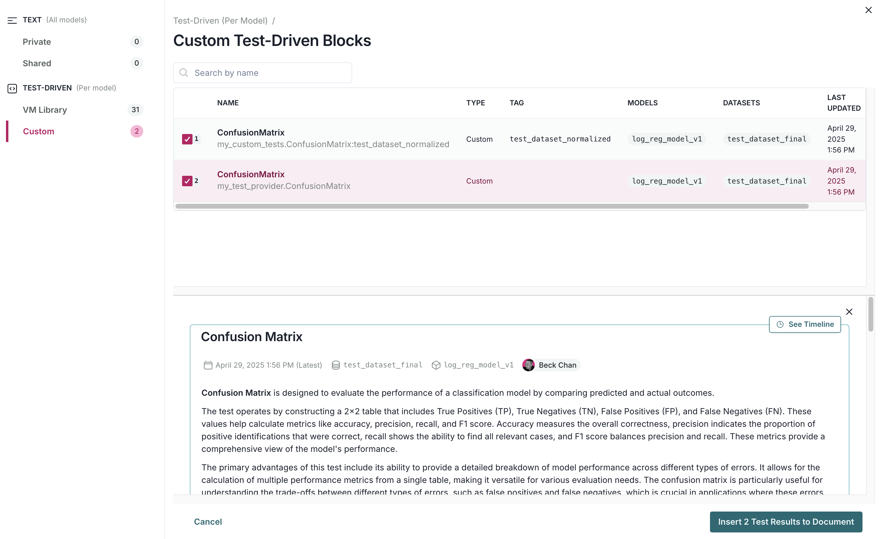
   • Select the two custom ConfusionMatrix tests you logged above:

   
   
   

6. Finally, click Insert 2 Test Results to Document to add the test results to the documentation.

   Confirm that the two individual results for the confusion matrix tests have been correctly inserted into section 3.2. Model Evaluation of the documentation.

In summary

In this third notebook, you learned how to:

• Implement a custom inline test
• Run and log your custom inline tests
• Use external custom test providers
• Run and log tests from your custom test providers

Next steps

Finalize testing and documentation

Now that you're proficient at using the ValidMind Library to run and log tests, let's put the last pieces in place to prepare our fully documented sample model for review: 4 — Finalize testing and documentation

---

Copyright © 2023-2026 ValidMind Inc. All rights reserved.
Refer to LICENSE for details.
SPDX-License-Identifier: AGPL-3.0 AND ValidMind Commercial