ValidMind for validation 4 — Finalize testing and reporting

Learn how to use ValidMind for your end-to-end validation process with our series of four introductory notebooks. In this last notebook, finalize the compliance assessment process and have a complete validation report ready for review.

This notebook will walk you through how to supplement ValidMind tests with your own custom tests and include them as additional evidence in your validation report. A custom test is any function that takes a set of inputs and parameters as arguments and returns one or more outputs:

• The function can be as simple or as complex as you need it to be — it can use external libraries, make API calls, or do anything else that you can do in Python.
• The only requirement is that the function signature and return values can be "understood" and handled by the ValidMind Library. As such, custom tests offer added flexibility by extending the default tests provided by ValidMind, enabling you to document any type of record (model) or use case.

For a more in-depth introduction to custom tests, refer to our Implement custom tests notebook.

Learn by doing

Our course tailor-made for validators new to ValidMind combines this series of notebooks with more a more in-depth introduction to the ValidMind Platform — Validator Fundamentals

Prerequisites

In order to finalize validation and reporting, you'll need to first have:

• Registered a model within the ValidMind Platform and granted yourself access to the model as a validator
• Installed the ValidMind Library in your local environment, allowing you to access all its features
• Learned how to import and initialize datasets and models for use with ValidMind
• Understood the basics of how to identify and run validation tests
• Run validation tests for your champion and challengers, and logged the results of those tests to the ValidMind Platform
• Inserted your logged test results into your validation report
• Added some preliminary artifacts (findings) to your validation report

Need help with the above steps?

Refer to the first three notebooks in this series:

• 1 — Set up the ValidMind Library for validation
• 2 — Start the validation process
• 3 — Developing a potential challenger

Setting up

This section should be very familiar to you now — as we performed the same actions in the previous two notebooks in this series.

Initialize the ValidMind Library

As usual, let's first connect up the ValidMind Library to our model we previously registered in the ValidMind Platform:

1. On the left sidebar that appears for your model, select Getting Started and select Validation from the Document drop-down menu.

2. Click Copy snippet to clipboard.

3. Next, load your model identifier credentials from an .env file or replace the placeholder with your own code snippet:

# Make sure the ValidMind Library is installed

%pip install -q validmind

# Load your model identifier credentials from an `.env` file

%load_ext dotenv
%dotenv .env

# Or replace with your code snippet

import validmind as vm

vm.init(
    # api_host="...",
    # api_key="...",
    # api_secret="...",
    # model="...",
    document="validation-report",
)

Note: you may need to restart the kernel to use updated packages.

2026-09-11 23:55:34,069 - INFO(validmind.api_client): 🎉 Connected to ValidMind!
📊 Model: [ValidMind Academy] Model validation (ID: cmalguc9y02ok199q2db381ib)
📁 Document Type: validation_report

Import the sample dataset

Next, we'll load in the same sample Bank Customer Churn Prediction dataset used to develop the champion that we will independently preprocess:

# Load the sample dataset
from validmind.datasets.classification import customer_churn as demo_dataset

print(
    f"Loaded demo dataset with: \n\n\t• Target column: '{demo_dataset.target_column}' \n\t• Class labels: {demo_dataset.class_labels}"
)

raw_df = demo_dataset.load_data()

Loaded demo dataset with: 

    • Target column: 'Exited' 
    • Class labels: {'0': 'Did not exit', '1': 'Exited'}

# Initialize the raw dataset for use in ValidMind tests
vm_raw_dataset = vm.init_dataset(
    dataset=raw_df,
    input_id="raw_dataset",
    target_column="Exited",
)

import pandas as pd

raw_copy_df = raw_df.sample(frac=1)  # Create a copy of the raw dataset

# Create a balanced dataset with the same number of exited and not exited customers
exited_df = raw_copy_df.loc[raw_copy_df["Exited"] == 1]
not_exited_df = raw_copy_df.loc[raw_copy_df["Exited"] == 0].sample(n=exited_df.shape[0])

balanced_raw_df = pd.concat([exited_df, not_exited_df])
balanced_raw_df = balanced_raw_df.sample(frac=1, random_state=42)

Let’s also quickly remove highly correlated features from the dataset using the output from a ValidMind test:

# Register new data and now 'balanced_raw_dataset' is the new dataset object of interest
vm_balanced_raw_dataset = vm.init_dataset(
    dataset=balanced_raw_df,
    input_id="balanced_raw_dataset",
    target_column="Exited",
)

# Run HighPearsonCorrelation test with our balanced dataset as input and return a result object
corr_result = vm.tests.run_test(
    test_id="validmind.data_validation.HighPearsonCorrelation",
    params={"max_threshold": 0.3},
    inputs={"dataset": vm_balanced_raw_dataset},
)

❌ High Pearson Correlation

The High Pearson Correlation test evaluates pairwise linear relationships among dataset features to identify highly correlated pairs that may indicate redundancy or multicollinearity. The results table reports the top 10 feature pairs ranked by Pearson correlation coefficient, alongside Pass/Fail status based on the configured absolute threshold of 0.3. Observed coefficients range from -0.1819 to 0.3496, with one pair exceeding the threshold and the remaining reported pairs falling below it.

Key insights:

• One pair exceeds threshold: The pair (Age, Exited) has a Pearson correlation coefficient of 0.3496, which is above the configured threshold of 0.3 and is therefore marked Fail.
• Remaining reported pairs are below threshold: The other nine reported feature pairs are marked Pass, with absolute correlation values ranging from 0.0338 to 0.1819, indicating weaker linear relationships within the reported set.
• Largest negative correlation is modest: The most negative reported coefficient is -0.1819 for (IsActiveMember, Exited), which remains below the threshold in absolute value.
• Reported correlations are concentrated near zero: Aside from (Age, Exited), all listed coefficients are relatively small in magnitude, including (Balance, NumOfProducts) at -0.1803 and (Balance, Exited) at 0.1563.

The reported correlation structure shows a single feature pair breaching the configured Pearson correlation threshold, while the rest of the top-ranked pairs remain below it. Within the reported results, linear dependence is limited in magnitude for most pairs, with coefficients clustered well under the threshold. This indicates that the observed high-correlation finding is concentrated in (Age, Exited) rather than broadly distributed across the listed feature relationships.

Parameters:

{
  "max_threshold": 0.3
}
            

Tables

Columns	Coefficient	Pass/Fail
(Age, Exited)	0.3496	Fail
(IsActiveMember, Exited)	-0.1819	Pass
(Balance, NumOfProducts)	-0.1803	Pass
(Balance, Exited)	0.1563	Pass
(NumOfProducts, Exited)	-0.0664	Pass
(NumOfProducts, IsActiveMember)	0.0515	Pass
(Balance, HasCrCard)	-0.0451	Pass
(Age, NumOfProducts)	-0.0411	Pass
(Balance, EstimatedSalary)	0.0376	Pass
(Tenure, IsActiveMember)	-0.0338	Pass

# From result object, extract table from `corr_result.tables`
features_df = corr_result.tables[0].data
features_df

	Columns	Coefficient	Pass/Fail
0	(Age, Exited)	0.3496	Fail
1	(IsActiveMember, Exited)	-0.1819	Pass
2	(Balance, NumOfProducts)	-0.1803	Pass
3	(Balance, Exited)	0.1563	Pass
4	(NumOfProducts, Exited)	-0.0664	Pass
5	(NumOfProducts, IsActiveMember)	0.0515	Pass
6	(Balance, HasCrCard)	-0.0451	Pass
7	(Age, NumOfProducts)	-0.0411	Pass
8	(Balance, EstimatedSalary)	0.0376	Pass
9	(Tenure, IsActiveMember)	-0.0338	Pass

# Extract list of features that failed the test
high_correlation_features = features_df[features_df["Pass/Fail"] == "Fail"]["Columns"].tolist()
high_correlation_features

['(Age, Exited)']

# Extract feature names from the list of strings
high_correlation_features = [feature.split(",")[0].strip("()") for feature in high_correlation_features]
high_correlation_features

['Age']

# Remove the highly correlated features from the dataset
balanced_raw_no_age_df = balanced_raw_df.drop(columns=high_correlation_features)

# Re-initialize the dataset object
vm_raw_dataset_preprocessed = vm.init_dataset(
    dataset=balanced_raw_no_age_df,
    input_id="raw_dataset_preprocessed",
    target_column="Exited",
)

# Re-run the test with the reduced feature set
corr_result = vm.tests.run_test(
    test_id="validmind.data_validation.HighPearsonCorrelation",
    params={"max_threshold": 0.3},
    inputs={"dataset": vm_raw_dataset_preprocessed},
)

✅ High Pearson Correlation

The High Pearson Correlation test evaluates linear relationships between feature pairs to identify potentially redundant variables or signs of multicollinearity. The result table reports the top pairwise Pearson correlation coefficients using a maximum threshold of 0.3, along with a Pass/Fail classification for each pair. The displayed coefficients range from -0.1819 to 0.1563 across the ten reported feature pairs. All reported pairs are classified as Pass under the configured threshold.

Key insights:

• No pair exceeds threshold: All reported absolute correlation coefficients are below the 0.3 threshold, and every listed feature pair is marked Pass.
• Largest observed relationship is modest: The strongest reported correlation is between IsActiveMember and Exited at -0.1819, which remains materially below the configured threshold.
• Top correlations are weak in magnitude: The next largest relationships are Balance with NumOfProducts at -0.1803 and Balance with Exited at 0.1563, with remaining reported coefficients closer to zero.
• Reported relationships include both directions: The table contains both negative and positive coefficients, indicating that the strongest observed linear associations in the reported set are mixed in direction rather than concentrated in one pattern.

The reported correlation structure does not show any feature pair with a linear relationship above the configured screening threshold. The strongest observed associations are modest in magnitude, and the remaining reported pairs are weaker still. Collectively, the test output indicates limited linear dependence among the listed top feature pairs under this Pearson correlation assessment.

Parameters:

{
  "max_threshold": 0.3
}
            

Tables

Columns	Coefficient	Pass/Fail
(IsActiveMember, Exited)	-0.1819	Pass
(Balance, NumOfProducts)	-0.1803	Pass
(Balance, Exited)	0.1563	Pass
(NumOfProducts, Exited)	-0.0664	Pass
(NumOfProducts, IsActiveMember)	0.0515	Pass
(Balance, HasCrCard)	-0.0451	Pass
(Balance, EstimatedSalary)	0.0376	Pass
(Tenure, IsActiveMember)	-0.0338	Pass
(Tenure, EstimatedSalary)	0.0324	Pass
(HasCrCard, IsActiveMember)	-0.0270	Pass

Split the preprocessed dataset

With our raw dataset rebalanced with highly correlated features removed, let's now spilt our dataset into train and test in preparation for model evaluation testing:

# Encode categorical features in the dataset
balanced_raw_no_age_df = pd.get_dummies(
    balanced_raw_no_age_df, columns=["Geography", "Gender"], drop_first=True
)
balanced_raw_no_age_df.head()

	CreditScore	Tenure	Balance	NumOfProducts	HasCrCard	IsActiveMember	EstimatedSalary	Exited	Geography_Germany	Geography_Spain	Gender_Male
2604	652	7	0.00	2	1	0	68789.93	0	False	True	True
1111	521	9	134504.78	1	1	0	18082.06	0	True	False	False
92	685	3	90536.81	1	0	1	63082.88	0	True	False	True
6099	723	3	110357.00	1	0	0	141977.54	1	True	False	False
1602	621	0	0.00	1	1	1	133831.37	1	False	False	True

from sklearn.model_selection import train_test_split

# Split the dataset into train and test
train_df, test_df = train_test_split(balanced_raw_no_age_df, test_size=0.20)

X_train = train_df.drop("Exited", axis=1)
y_train = train_df["Exited"]
X_test = test_df.drop("Exited", axis=1)
y_test = test_df["Exited"]

# Initialize the split datasets
vm_train_ds = vm.init_dataset(
    input_id="train_dataset_final",
    dataset=train_df,
    target_column="Exited",
)

vm_test_ds = vm.init_dataset(
    input_id="test_dataset_final",
    dataset=test_df,
    target_column="Exited",
)

Import the champion model

With our raw dataset assessed and preprocessed, let's go ahead and import the champion submitted by the development team in the format of a .pkl file: lr_model_champion.pkl

# Import the champion model
import pickle as pkl

with open("lr_model_champion.pkl", "rb") as f:
    log_reg = pkl.load(f)

/opt/hostedtoolcache/Python/3.11.16/x64/lib/python3.11/site-packages/sklearn/base.py:442: InconsistentVersionWarning: Trying to unpickle estimator LogisticRegression from version 1.3.2 when using version 1.7.2. This might lead to breaking code or invalid results. Use at your own risk. For more info please refer to:
https://scikit-learn.org/stable/model_persistence.html#security-maintainability-limitations
  warnings.warn(

Train potential challenger model

We'll also train our random forest classification challenger to see how it compares:

# Import the Random Forest Classification model
from sklearn.ensemble import RandomForestClassifier

# Create the model instance with 50 decision trees
rf_model = RandomForestClassifier(
    n_estimators=50,
    random_state=42,
)

# Train the model
rf_model.fit(X_train, y_train)

RandomForestClassifier(n_estimators=50, random_state=42)

In a Jupyter environment, please rerun this cell to show the HTML representation or trust the notebook.
On GitHub, the HTML representation is unable to render, please try loading this page with nbviewer.org.

Initialize the ValidMind models

In addition to the initialized datasets, you'll also need to initialize a ValidMind model object (vm_model) that can be passed to other functions for analysis and tests on the data for each of our two models:

# Initialize the champion logistic regression model
vm_log_model = vm.init_model(
    log_reg,
    input_id="log_model_champion",
)

# Initialize the challenger random forest classification model
vm_rf_model = vm.init_model(
    rf_model,
    input_id="rf_model",
)

# Assign predictions to Champion — Logistic regression model
vm_train_ds.assign_predictions(model=vm_log_model)
vm_test_ds.assign_predictions(model=vm_log_model)

# Assign predictions to Challenger — Random forest classification model
vm_train_ds.assign_predictions(model=vm_rf_model)
vm_test_ds.assign_predictions(model=vm_rf_model)

2026-09-11 23:55:43,278 - INFO(validmind.vm_models.dataset.utils): Running predict_proba()... This may take a while
2026-09-11 23:55:43,279 - INFO(validmind.vm_models.dataset.utils): Done running predict_proba()
2026-09-11 23:55:43,280 - INFO(validmind.vm_models.dataset.utils): Running predict()... This may take a while
2026-09-11 23:55:43,282 - INFO(validmind.vm_models.dataset.utils): Done running predict()
2026-09-11 23:55:43,283 - INFO(validmind.vm_models.dataset.utils): Running predict_proba()... This may take a while
2026-09-11 23:55:43,284 - INFO(validmind.vm_models.dataset.utils): Done running predict_proba()
2026-09-11 23:55:43,285 - INFO(validmind.vm_models.dataset.utils): Running predict()... This may take a while
2026-09-11 23:55:43,285 - INFO(validmind.vm_models.dataset.utils): Done running predict()
2026-09-11 23:55:43,287 - INFO(validmind.vm_models.dataset.utils): Running predict_proba()... This may take a while
2026-09-11 23:55:43,305 - INFO(validmind.vm_models.dataset.utils): Done running predict_proba()
2026-09-11 23:55:43,306 - INFO(validmind.vm_models.dataset.utils): Running predict()... This may take a while
2026-09-11 23:55:43,323 - INFO(validmind.vm_models.dataset.utils): Done running predict()
2026-09-11 23:55:43,325 - INFO(validmind.vm_models.dataset.utils): Running predict_proba()... This may take a while
2026-09-11 23:55:43,332 - INFO(validmind.vm_models.dataset.utils): Done running predict_proba()
2026-09-11 23:55:43,332 - INFO(validmind.vm_models.dataset.utils): Running predict()... This may take a while
2026-09-11 23:55:43,339 - INFO(validmind.vm_models.dataset.utils): Done running predict()

Implementing custom tests

Thanks to the documentation (Learn more: ValidMind for development), we know that the development team implemented a custom test to further evaluate the performance of the champion.

In a usual validation situation, you would load a saved custom test provided by the development team. In the following section, we'll have you implement the same custom test and make it available for reuse, to familiarize you with the processes.

Want to learn more about custom tests?

Refer to our in-depth introduction to custom tests: Implement custom tests

Implement a custom inline test

Let's implement the same custom inline test that calculates the confusion matrix for a binary classification model that the development team used in their performance evaluations.

• An inline test refers to a test written and executed within the same environment as the code being tested — in this case, right in this Jupyter Notebook — without requiring a separate test file or framework.
• You'll note that the custom test function is just a regular Python function that can include and require any Python library as you see fit.

Create a confusion matrix plot

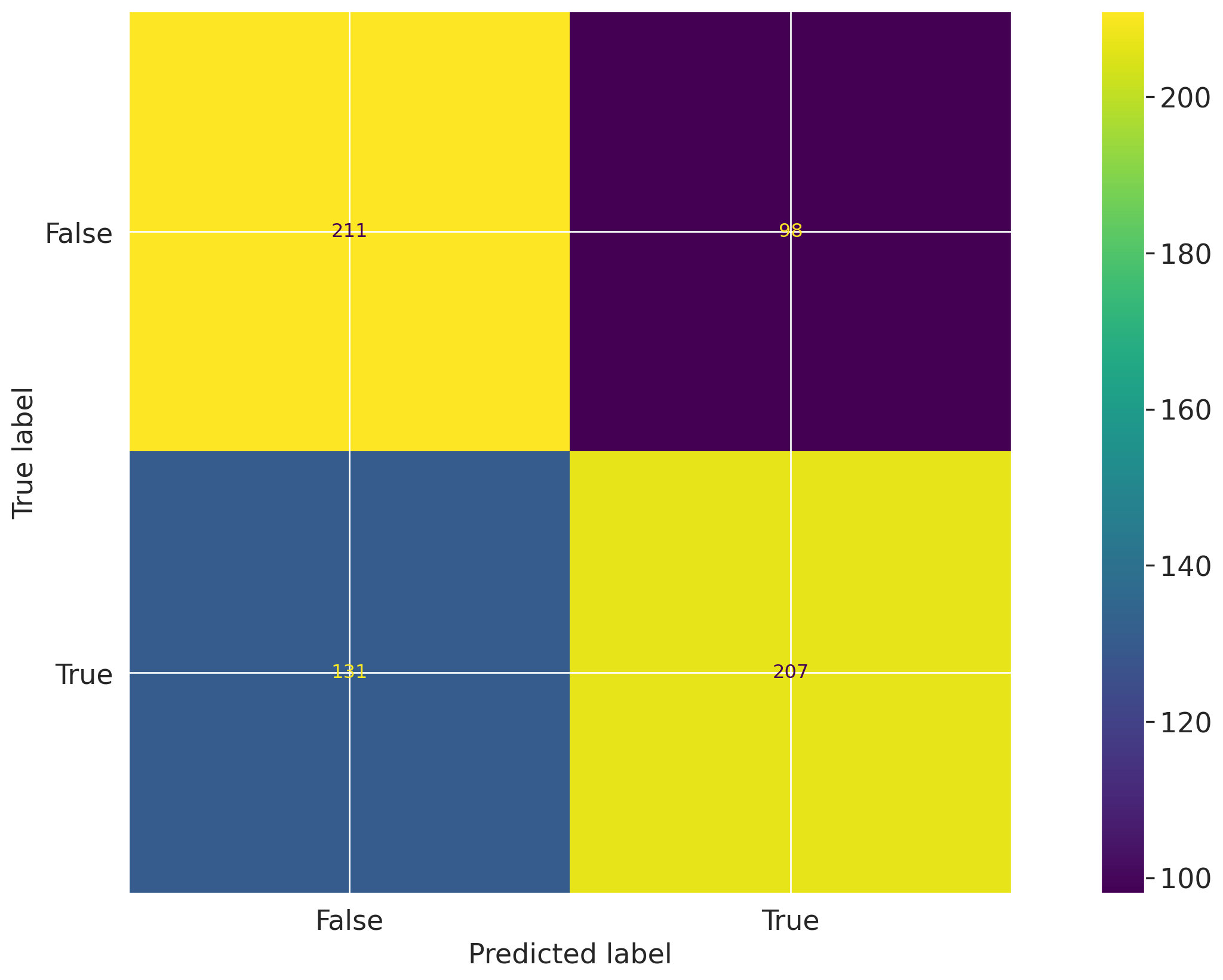
Let's first create a confusion matrix plot using the confusion_matrix function from the sklearn.metrics module:

import matplotlib.pyplot as plt
from sklearn import metrics

# Get the predicted classes
y_pred = log_reg.predict(vm_test_ds.x)

confusion_matrix = metrics.confusion_matrix(y_test, y_pred)

cm_display = metrics.ConfusionMatrixDisplay(
    confusion_matrix=confusion_matrix, display_labels=[False, True]
)
cm_display.plot()

Next, create a @vm.test wrapper that will allow you to create a reusable test. Note the following changes in the code below:

• The function confusion_matrix takes two arguments dataset and model. This is a VMDataset and VMModel object respectively.
  • VMDataset objects allow you to access the dataset's true (target) values by accessing the .y attribute.
  • VMDataset objects allow you to access the predictions for a given record (model) by accessing the .y_pred() method.
• The function docstring provides a description of what the test does. This will be displayed along with the result in this notebook as well as in the ValidMind Platform.
• The function body calculates the confusion matrix using the sklearn.metrics.confusion_matrix function as we just did above.
• The function then returns the ConfusionMatrixDisplay.figure_ object — this is important as the ValidMind Library expects the output of the custom test to be a plot or a table.
• The @vm.test decorator is doing the work of creating a wrapper around the function that will allow it to be run by the ValidMind Library. It also registers the test so it can be found by the ID my_custom_tests.ConfusionMatrix.

@vm.test("my_custom_tests.ConfusionMatrix")
def confusion_matrix(dataset, model):
    """The confusion matrix is a table that is often used to describe the performance of a classification model on a set of data for which the true values are known.

    The confusion matrix is a 2x2 table that contains 4 values:

    - True Positive (TP): the number of correct positive predictions
    - True Negative (TN): the number of correct negative predictions
    - False Positive (FP): the number of incorrect positive predictions
    - False Negative (FN): the number of incorrect negative predictions

    The confusion matrix can be used to assess the holistic performance of a classification model by showing the accuracy, precision, recall, and F1 score of the model on a single figure.
    """
    y_true = dataset.y
    y_pred = dataset.y_pred(model=model)

    confusion_matrix = metrics.confusion_matrix(y_true, y_pred)

    cm_display = metrics.ConfusionMatrixDisplay(
        confusion_matrix=confusion_matrix, display_labels=[False, True]
    )
    cm_display.plot()

    plt.close()  # close the plot to avoid displaying it

    return cm_display.figure_  # return the figure object itself

You can now run the newly created custom test on both the training and test datasets for both models using the run_test() function:

# Champion train and test
vm.tests.run_test(
    test_id="my_custom_tests.ConfusionMatrix:champion",
    input_grid={
        "dataset": [vm_train_ds,vm_test_ds],
        "model" : [vm_log_model]
    }
).log()

Confusion Matrix Champion

The ConfusionMatrix test evaluates classification performance by comparing predicted labels against true labels across the training and test datasets. The result is presented as two 2×2 confusion matrices with counts for true negatives, false positives, false negatives, and true positives. For the training dataset, the matrix shows 828 true negatives, 468 false positives, 498 false negatives, and 791 true positives. For the test dataset, the matrix shows 201 true negatives, 119 false positives, 109 false negatives, and 218 true positives.

Key insights:

• Correct classifications exceed errors: In both datasets, the sum of diagonal cells is larger than the sum of off-diagonal cells. Training data contains 1,619 correct classifications versus 966 misclassifications, while test data contains 419 correct classifications versus 228 misclassifications.

• Negative class is identified more often correctly: True negatives exceed false positives in both datasets. The training matrix shows 828 true negatives versus 468 false positives, and the test matrix shows 201 true negatives versus 119 false positives.

• Positive class is also captured more often correctly: True positives exceed false negatives in both datasets. The training matrix shows 791 true positives versus 498 false negatives, and the test matrix shows 218 true positives versus 109 false negatives.

• Train and test error patterns are directionally similar: Both matrices show the same ordering in cell magnitudes, with correct classifications larger than the corresponding error counts for each class. In both datasets, false positives are slightly higher than false negatives.

The confusion matrices show that the model produces more correct than incorrect classifications on both the training and test datasets. For both the negative and positive classes, correct predictions exceed the corresponding error counts. The training and test results display a similar distribution of outcomes, with false positives remaining slightly more frequent than false negatives in each dataset.

Figures

2026-09-11 23:55:48,811 - INFO(validmind.vm_models.result.result): Test driven block with result_id my_custom_tests.ConfusionMatrix:champion does not exist in model's document

# Challenger train and test
vm.tests.run_test(
    test_id="my_custom_tests.ConfusionMatrix:challenger",
    input_grid={
        "dataset": [vm_train_ds,vm_test_ds],
        "model" : [vm_rf_model]
    }
).log()

Confusion Matrix Challenger

The Confusion Matrix test evaluates classification performance by comparing predicted labels with true labels and summarizing outcomes as true positives, true negatives, false positives, and false negatives. The result is shown separately for the training dataset and the test dataset. On the training dataset, the matrix contains 1,296 true negatives, 1,288 true positives, 0 false positives, and 1 false negative. On the test dataset, the matrix contains 237 true negatives, 231 true positives, 83 false positives, and 96 false negatives.

Key insights:

• Near-perfect training classification: The training confusion matrix shows 1,296 true negatives and 1,288 true positives, with only 1 false negative and 0 false positives. Misclassification on the training sample is therefore minimal.

• Test errors in both classes: The test confusion matrix shows errors in both directions, with 83 false positives and 96 false negatives. Correct classifications remain higher than incorrect classifications in both actual classes, but the gap is materially narrower than in training.

• Stronger separation in training than test: The transition from 1 total training error to 179 total test errors indicates substantially different classification outcomes across the two datasets. This difference is visible in both the negative class and the positive class.

The confusion matrices show that the challenger model classifies the training sample almost perfectly, while test-sample performance is materially less accurate and includes both false positive and false negative errors. Correct predictions remain the largest counts on the test dataset, but the contrast with the training matrix indicates a pronounced reduction in out-of-sample classification performance. The observed pattern is driven by the increase in both types of test misclassification relative to the training results.

Figures

2026-09-11 23:55:54,508 - INFO(validmind.vm_models.result.result): Test driven block with result_id my_custom_tests.ConfusionMatrix:challenger does not exist in model's document

Note the output returned indicating that a test-driven block doesn't currently exist in your documentation for some test IDs.

That's expected, as when we run validations tests the results logged need to be manually added to your report as part of your compliance assessment process within the ValidMind Platform.

Add parameters to custom tests

Custom tests can take parameters just like any other function. To demonstrate, let's modify the confusion_matrix function to take an additional parameter normalize that will allow you to normalize the confusion matrix:

@vm.test("my_custom_tests.ConfusionMatrix")
def confusion_matrix(dataset, model, normalize=False):
    """The confusion matrix is a table that is often used to describe the performance of a classification model on a set of data for which the true values are known.

    The confusion matrix is a 2x2 table that contains 4 values:

    - True Positive (TP): the number of correct positive predictions
    - True Negative (TN): the number of correct negative predictions
    - False Positive (FP): the number of incorrect positive predictions
    - False Negative (FN): the number of incorrect negative predictions

    The confusion matrix can be used to assess the holistic performance of a classification model by showing the accuracy, precision, recall, and F1 score of the model on a single figure.
    """
    y_true = dataset.y
    y_pred = dataset.y_pred(model=model)

    if normalize:
        confusion_matrix = metrics.confusion_matrix(y_true, y_pred, normalize="all")
    else:
        confusion_matrix = metrics.confusion_matrix(y_true, y_pred)

    cm_display = metrics.ConfusionMatrixDisplay(
        confusion_matrix=confusion_matrix, display_labels=[False, True]
    )
    cm_display.plot()

    plt.close()  # close the plot to avoid displaying it

    return cm_display.figure_  # return the figure object itself

Pass parameters to custom tests

You can pass parameters to custom tests by providing a dictionary of parameters to the run_test() function.

• The parameters will override any default parameters set in the custom test definition. Note that dataset and model are still passed as inputs.
• Since these are VMDataset or VMModel inputs, they have a special meaning.

Re-running and logging the custom confusion matrix with normalize=True for both models and our testing dataset looks like this:

# Champion with test dataset and normalize=True
vm.tests.run_test(
    test_id="my_custom_tests.ConfusionMatrix:test_normalized_champion",
    input_grid={
        "dataset": [vm_test_ds],
        "model" : [vm_log_model]
    },
    params={"normalize": True}
).log()

Confusion Matrix Test Normalized Champion

The ConfusionMatrix test evaluates classification outcomes by comparing predicted labels against true labels, and this result presents the normalized confusion matrix for log_model_champion on test_dataset_final. The matrix is shown as a 2x2 heatmap with normalized cell values, where rows correspond to true labels and columns correspond to predicted labels. The observed cell values are 0.31 for true negatives, 0.18 for false positives, 0.17 for false negatives, and 0.34 for true positives.

Key insights:

• Correct classifications total 0.65: The diagonal cells sum to 0.65, with 0.31 in the true negative cell and 0.34 in the true positive cell, indicating that normalized correct predictions exceed misclassifications.
• True positives are the largest cell: The highest normalized value in the matrix is 0.34 for cases with true label True and predicted label True, making this the single largest outcome category.
• False positives slightly exceed false negatives: Misclassifications are split between 0.18 false positives and 0.17 false negatives, showing a nearly balanced error pattern with a marginally higher false positive share.
• Prediction outcomes are relatively balanced: The four normalized cell values range from 0.17 to 0.34, with no cell showing extreme concentration relative to the others.

The normalized confusion matrix shows that correct classifications account for 0.65 of all observations, with slightly more true positives than true negatives. Misclassifications account for 0.35 of observations and are distributed almost evenly between false positives and false negatives. Overall, the result reflects a relatively balanced distribution across the four outcome categories, with the largest share concentrated in true positive predictions.

Parameters:

{
  "normalize": true
}
            

Figures

2026-09-11 23:55:59,518 - INFO(validmind.vm_models.result.result): Test driven block with result_id my_custom_tests.ConfusionMatrix:test_normalized_champion does not exist in model's document

# Challenger with test dataset and normalize=True
vm.tests.run_test(
    test_id="my_custom_tests.ConfusionMatrix:test_normalized_challenger",
    input_grid={
        "dataset": [vm_test_ds],
        "model" : [vm_rf_model]
    },
    params={"normalize": True}
).log()

Confusion Matrix Test Normalized Challenger

The ConfusionMatrix:test_normalized_challenger test evaluates classification performance by comparing predicted labels against true labels in a normalized 2x2 confusion matrix. The result is shown for dataset=test_dataset_final and model=rf_model, with normalization enabled. The matrix reports proportions across the four outcome cells: 0.37 for true negatives, 0.13 for false positives, 0.15 for false negatives, and 0.36 for true positives.

Key insights:

• Correct classifications dominate: The diagonal cells sum to 0.73, comprising 0.37 true negatives and 0.36 true positives, while the off-diagonal cells sum to 0.28 based on the displayed rounded values.
• Negative-class errors are lower: False positives account for 0.13 of observations, which is lower than the 0.37 true negative share within the true negative row.
• Positive-class errors are moderate: False negatives account for 0.15 of observations, compared with 0.36 true positives in the true positive row.
• Class outcomes appear balanced: The two correct classification cells are similar in magnitude, with 0.37 for true negatives and 0.36 for true positives.

The normalized confusion matrix indicates that most observations fall on the diagonal, reflecting a larger share of correct than incorrect classifications. Correct identification is distributed similarly across the negative and positive classes, with true negative and true positive proportions of 0.37 and 0.36, respectively. Misclassifications are present in both directions, with false negatives at 0.15 and false positives at 0.13.

Parameters:

{
  "normalize": true
}
            

Figures

2026-09-11 23:56:04,386 - INFO(validmind.vm_models.result.result): Test driven block with result_id my_custom_tests.ConfusionMatrix:test_normalized_challenger does not exist in model's document

Use external test providers

Sometimes you may want to reuse the same set of custom tests across multiple records (models) and share them with others in your organization, like the development team would have done with you in this example workflow featured in this series of notebooks. In this case, you can create an external custom test provider that will allow you to load custom tests from a local folder or a Git repository.

In this section you will learn how to declare a local filesystem test provider that allows loading tests from a local folder following these high level steps:

1. Create a folder of custom tests from existing inline tests (tests that exist in your active Jupyter Notebook)
2. Save an inline test to a file
3. Define and register a LocalTestProvider that points to that folder
4. Run test provider tests
5. Add the test results to your documentation

Create custom tests folder

Let's start by creating a new folder that will contain reusable custom tests from your existing inline tests.

The following code snippet will create a new my_tests directory in the current working directory if it doesn't exist:

tests_folder = "my_tests"

import os

# create tests folder
os.makedirs(tests_folder, exist_ok=True)

# remove existing tests
for f in os.listdir(tests_folder):
    # remove files and pycache
    if f.endswith(".py") or f == "__pycache__":
        os.system(f"rm -rf {tests_folder}/{f}")

After running the command above, confirm that a new my_tests directory was created successfully. For example:

~/notebooks/tutorials/validation/my_tests/

Save an inline test

The @vm.test decorator we used in Implement a custom inline test above to register one-off custom tests also includes a convenience method on the function object that allows you to simply call <func_name>.save() to save the test to a Python file at a specified path.

While save() will get you started by creating the file and saving the function code with the correct name, it won't automatically include any imports, or other functions or variables, outside of the functions that are needed for the test to run. To solve this, pass in an optional imports argument ensuring necessary imports are added to the file.

The confusion_matrix test requires the following additional imports:

import matplotlib.pyplot as plt
from sklearn import metrics

Let's pass these imports to the save() method to ensure they are included in the file with the following command:

confusion_matrix.save(
    # Save it to the custom tests folder we created
    tests_folder,
    imports=["import matplotlib.pyplot as plt", "from sklearn import metrics"],
)

2026-09-11 23:56:04,846 - INFO(validmind.tests.decorator): Saved to /home/runner/work/documentation/documentation/site/notebooks/EXECUTED/validation/my_tests/ConfusionMatrix.py!Be sure to add any necessary imports to the top of the file.
2026-09-11 23:56:04,847 - INFO(validmind.tests.decorator): This metric can be run with the ID: <test_provider_namespace>.ConfusionMatrix

• Confirm that the save() method saved the confusion_matrix function to a file named ConfusionMatrix.py in the my_tests folder.

• Note that the new file provides some context on the origin of the test, which is useful for traceability:

  # Saved from __main__.confusion_matrix
  # Original Test ID: my_custom_tests.ConfusionMatrix
  # New Test ID: <test_provider_namespace>.ConfusionMatrix

• Additionally, the new test function has been stripped off its decorator, as it now resides in a file that will be loaded by the test provider:

  def ConfusionMatrix(dataset, model, normalize=False):

Register a local test provider

Now that your my_tests folder has a sample custom test, let's initialize a test provider that will tell the ValidMind Library where to find your custom tests:

• ValidMind offers out-of-the-box test providers for local tests (tests in a folder) or a Github provider for tests in a Github repository.
• You can also create your own test provider by creating a class that has a load_test method that takes a test ID and returns the test function matching that ID.

Want to learn more about test providers?

An extended introduction to test providers can be found in: Integrate external test providers

Initialize a local test provider

For most use cases, using a LocalTestProvider that allows you to load custom tests from a designated directory should be sufficient.

The most important attribute for a test provider is its namespace. This is a string that will be used to prefix test IDs in documentation. This allows you to have multiple test providers with tests that can even share the same ID, but are distinguished by their namespace.

Let's go ahead and load the custom tests from our my_tests directory:

from validmind.tests import LocalTestProvider

# initialize the test provider with the tests folder we created earlier
my_test_provider = LocalTestProvider(tests_folder)

vm.tests.register_test_provider(
    namespace="my_test_provider",
    test_provider=my_test_provider,
)
# `my_test_provider.load_test()` will be called for any test ID that starts with `my_test_provider`
# e.g. `my_test_provider.ConfusionMatrix` will look for a function named `ConfusionMatrix` in `my_tests/ConfusionMatrix.py` file

Run test provider tests

Now that we've set up the test provider, we can run any test that's located in the tests folder by using the run_test() method as with any other test:

• For tests that reside in a test provider directory, the test ID will be the namespace specified when registering the provider, followed by the path to the test file relative to the tests folder.
• For example, the Confusion Matrix test we created earlier will have the test ID my_test_provider.ConfusionMatrix. You could organize the tests in subfolders, say classification and regression, and the test ID for the Confusion Matrix test would then be my_test_provider.classification.ConfusionMatrix.

Let's go ahead and re-run the confusion matrix test with our testing dataset for our two models by using the test ID my_test_provider.ConfusionMatrix. This should load the test from the test provider and run it as before.

# Champion with test dataset and test provider custom test
vm.tests.run_test(
    test_id="my_test_provider.ConfusionMatrix:champion",
    input_grid={
        "dataset": [vm_test_ds],
        "model" : [vm_log_model]
    }
).log()

Confusion Matrix Champion

The Confusion Matrix test evaluates classification performance by comparing predicted labels with observed labels across the test dataset. The matrix for test_dataset_final and log_model_champion reports counts for correct and incorrect classifications in each outcome category. The four cells show 201 observations with true label False predicted as False, 119 observations with true label False predicted as True, 109 observations with true label True predicted as False, and 218 observations with true label True predicted as True.

Key insights:

• Correct classifications exceed errors: The diagonal cells contain 201 true negatives and 218 true positives, for a combined 419 correct classifications, compared with 228 misclassifications from the off-diagonal cells.
• True positives are the largest cell: The highest single count in the matrix is 218 for observations with true label True predicted as True, indicating the most frequent outcome is correct identification of the positive class.
• False positives slightly exceed false negatives: Misclassifications are split between 119 false positives and 109 false negatives, showing a small imbalance toward predicting True when the observed label is False.
• Class outcomes are relatively balanced: Observed labels total 320 for False cases and 327 for True cases, while predicted labels total 310 for False predictions and 337 for True predictions.

The confusion matrix shows that correct classifications are concentrated on the diagonal, with true positives and true negatives both materially larger than either error cell. Misclassifications are present in both directions and are of similar magnitude, with false positives marginally higher than false negatives. Overall, the result reflects a relatively balanced distribution across observed and predicted classes with more correct than incorrect classifications.

Figures

2026-09-11 23:56:09,721 - INFO(validmind.vm_models.result.result): Test driven block with result_id my_test_provider.ConfusionMatrix:champion does not exist in model's document

# Challenger with test dataset  and test provider custom test
vm.tests.run_test(
    test_id="my_test_provider.ConfusionMatrix:challenger",
    input_grid={
        "dataset": [vm_test_ds],
        "model" : [vm_rf_model]
    }
).log()

Confusion Matrix Challenger

The Confusion Matrix test evaluates classification performance by comparing predicted labels with observed labels. The result is presented as a 2×2 matrix for the rf_model on test_dataset_final, with counts for true negatives, false positives, false negatives, and true positives. The matrix shows 237 observations in the true negative cell, 83 in the false positive cell, 96 in the false negative cell, and 231 in the true positive cell. These counts provide the basis for assessing how predictions are distributed across correct and incorrect classifications.

Key insights:

• Correct classifications exceed errors: The diagonal cells contain 237 true negatives and 231 true positives, for a combined 468 correct classifications, compared with 179 total misclassifications from 83 false positives and 96 false negatives.

• Error types are relatively balanced: False negatives total 96 and false positives total 83. The difference between the two error counts is 13, indicating that neither error type dominates the confusion matrix.

• Negative and positive classes show similar correct counts: Correct predictions are similar across classes, with 237 true negatives versus 231 true positives. This indicates a closely balanced distribution of correct outcomes between the two classes.

The confusion matrix shows that most observations were classified correctly, with correct predictions concentrated in both diagonal cells at similar levels. Misclassifications are present in both directions, and the counts of false positives and false negatives are comparatively close. Overall, the result reflects a relatively balanced classification pattern across the positive and negative classes.

Figures

2026-09-11 23:56:14,175 - INFO(validmind.vm_models.result.result): Test driven block with result_id my_test_provider.ConfusionMatrix:challenger does not exist in model's document

Verify test runs

Our final task is to verify that all the tests provided by the development team were run and reported accurately. Note the appended result_ids to delineate which dataset we ran the test with for the relevant tests.

Here, we'll specify all the tests we'd like to independently rerun in a dictionary called test_config. Note here that inputs and input_grid expect the input_id of the dataset or model as the value rather than the variable name we specified:

test_config = {
    # Run with the raw dataset
    'validmind.data_validation.DatasetDescription:raw_data': {
        'inputs': {'dataset': 'raw_dataset'}
    },
    'validmind.data_validation.DescriptiveStatistics:raw_data': {
        'inputs': {'dataset': 'raw_dataset'}
    },
    'validmind.data_validation.MissingValues:raw_data': {
        'inputs': {'dataset': 'raw_dataset'},
        'params': {'min_percentage_threshold': 1}
    },
    'validmind.data_validation.ClassImbalance:raw_data': {
        'inputs': {'dataset': 'raw_dataset'},
        'params': {'min_percent_threshold': 10}
    },
    'validmind.data_validation.Duplicates:raw_data': {
        'inputs': {'dataset': 'raw_dataset'},
        'params': {'min_threshold': 1}
    },
    'validmind.data_validation.HighCardinality:raw_data': {
        'inputs': {'dataset': 'raw_dataset'},
        'params': {
            'num_threshold': 100,
            'percent_threshold': 0.1,
            'threshold_type': 'percent'
        }
    },
    'validmind.data_validation.Skewness:raw_data': {
        'inputs': {'dataset': 'raw_dataset'},
        'params': {'max_threshold': 1}
    },
    'validmind.data_validation.UniqueRows:raw_data': {
        'inputs': {'dataset': 'raw_dataset'},
        'params': {'min_percent_threshold': 1}
    },
    'validmind.data_validation.TooManyZeroValues:raw_data': {
        'inputs': {'dataset': 'raw_dataset'},
        'params': {'max_percent_threshold': 0.03}
    },
    'validmind.data_validation.IQROutliersTable:raw_data': {
        'inputs': {'dataset': 'raw_dataset'},
        'params': {'threshold': 5}
    },
    # Run with the preprocessed dataset
    'validmind.data_validation.DescriptiveStatistics:preprocessed_data': {
        'inputs': {'dataset': 'raw_dataset_preprocessed'}
    },
    'validmind.data_validation.TabularDescriptionTables:preprocessed_data': {
        'inputs': {'dataset': 'raw_dataset_preprocessed'}
    },
    'validmind.data_validation.MissingValues:preprocessed_data': {
        'inputs': {'dataset': 'raw_dataset_preprocessed'},
        'params': {'min_percentage_threshold': 1}
    },
    'validmind.data_validation.TabularNumericalHistograms:preprocessed_data': {
        'inputs': {'dataset': 'raw_dataset_preprocessed'}
    },
    'validmind.data_validation.TabularCategoricalBarPlots:preprocessed_data': {
        'inputs': {'dataset': 'raw_dataset_preprocessed'}
    },
    'validmind.data_validation.TargetRateBarPlots:preprocessed_data': {
        'inputs': {'dataset': 'raw_dataset_preprocessed'},
        'params': {'default_column': 'loan_status'}
    },
    # Run with the training and test datasets
    'validmind.data_validation.DescriptiveStatistics:development_data': {
        'input_grid': {'dataset': ['train_dataset_final', 'test_dataset_final']}
    },
    'validmind.data_validation.TabularDescriptionTables:development_data': {
        'input_grid': {'dataset': ['train_dataset_final', 'test_dataset_final']}
    },
    'validmind.data_validation.ClassImbalance:development_data': {
        'input_grid': {'dataset': ['train_dataset_final', 'test_dataset_final']},
        'params': {'min_percent_threshold': 10}
    },
    'validmind.data_validation.UniqueRows:development_data': {
        'input_grid': {'dataset': ['train_dataset_final', 'test_dataset_final']},
        'params': {'min_percent_threshold': 1}
    },
    'validmind.data_validation.TabularNumericalHistograms:development_data': {
        'input_grid': {'dataset': ['train_dataset_final', 'test_dataset_final']}
    },
    'validmind.data_validation.MutualInformation:development_data': {
        'input_grid': {'dataset': ['train_dataset_final', 'test_dataset_final']},
        'params': {'min_threshold': 0.01}
    },
    'validmind.data_validation.PearsonCorrelationMatrix:development_data': {
        'input_grid': {'dataset': ['train_dataset_final', 'test_dataset_final']}
    },
    'validmind.data_validation.HighPearsonCorrelation:development_data': {
        'input_grid': {'dataset': ['train_dataset_final', 'test_dataset_final']},
        'params': {'max_threshold': 0.3, 'top_n_correlations': 10}
    },
    'validmind.model_validation.ModelMetadata': {
        'input_grid': {'model': ['log_model_champion', 'rf_model']}
    },
    'validmind.model_validation.sklearn.ModelParameters': {
        'input_grid': {'model': ['log_model_champion', 'rf_model']}
    },
    'validmind.model_validation.sklearn.ROCCurve': {
        'input_grid': {'dataset': ['train_dataset_final', 'test_dataset_final'], 'model': ['log_model_champion']}
    },
    'validmind.model_validation.sklearn.MinimumROCAUCScore': {
        'input_grid': {'dataset': ['train_dataset_final', 'test_dataset_final'], 'model': ['log_model_champion']},
        'params': {'min_threshold': 0.5}
    }
}

Then batch run and log our tests in test_config:

for t in test_config:
    print(t)
    try:
        # Check if test has input_grid
        if 'input_grid' in test_config[t]:
            # For tests with input_grid, pass the input_grid configuration
            if 'params' in test_config[t]:
                vm.tests.run_test(t, input_grid=test_config[t]['input_grid'], params=test_config[t]['params']).log()
            else:
                vm.tests.run_test(t, input_grid=test_config[t]['input_grid']).log()
        else:
            # Original logic for regular inputs
            if 'params' in test_config[t]:
                vm.tests.run_test(t, inputs=test_config[t]['inputs'], params=test_config[t]['params']).log()
            else:
                vm.tests.run_test(t, inputs=test_config[t]['inputs']).log()
    except Exception as e:
        print(f"Error running test {t}: {str(e)}")

validmind.data_validation.DatasetDescription:raw_data

Dataset Description Raw Data

The Dataset Description test evaluates the structure, completeness, and basic cardinality of each column in the raw dataset. The result summarizes 11 variables across numeric and categorical types, reporting counts, missingness, and distinct-value levels for each field. All listed columns contain 8,000 observations with no missing values, and the table highlights variation in feature cardinality ranging from binary categorical fields to fully unique numeric values.

Key insights:

• No missing values across columns: All 11 variables report a count of 8,000 and missingness of 0.0%, indicating complete population coverage in the raw dataset summary.

• Mixed numeric and categorical structure: The dataset contains numeric variables (CreditScore, Age, Tenure, Balance, NumOfProducts, EstimatedSalary) and categorical variables (Geography, Gender, HasCrCard, IsActiveMember, Exited), reflecting a mixed feature set in the raw data.

• EstimatedSalary is fully unique: EstimatedSalary has 8,000 distinct values out of 8,000 observations, corresponding to a distinct ratio of 1.0, making it the highest-cardinality field in the dataset.

• Balance also shows high cardinality: Balance has 5,088 distinct values, representing 63.6% of observations, which is materially higher than the distinct-value levels of the other non-unique variables.

• Several variables have very low cardinality: Geography has 3 distinct values, Gender, HasCrCard, IsActiveMember, and Exited each have 2, and NumOfProducts has 4, indicating multiple fields with a small number of discrete states.

The raw dataset summary indicates complete records across all reported variables, with no observed missingness in any column. The feature set combines low-cardinality categorical fields with numeric variables that vary substantially in distinct-value concentration, most notably EstimatedSalary and Balance. Overall, the result describes a structurally complete dataset with a broad spread of feature cardinality across columns.

Tables

Dataset Description

Name	Type	Count	Missing	Missing %	Distinct	Distinct %
CreditScore	Numeric	8000.0	0	0.0	452	0.0565
Geography	Categorical	8000.0	0	0.0	3	0.0004
Gender	Categorical	8000.0	0	0.0	2	0.0002
Age	Numeric	8000.0	0	0.0	69	0.0086
Tenure	Numeric	8000.0	0	0.0	11	0.0014
Balance	Numeric	8000.0	0	0.0	5088	0.6360
NumOfProducts	Numeric	8000.0	0	0.0	4	0.0005
HasCrCard	Categorical	8000.0	0	0.0	2	0.0002
IsActiveMember	Categorical	8000.0	0	0.0	2	0.0002
EstimatedSalary	Numeric	8000.0	0	0.0	8000	1.0000
Exited	Categorical	8000.0	0	0.0	2	0.0002

2026-09-11 23:56:19,233 - INFO(validmind.vm_models.result.result): Test driven block with result_id validmind.data_validation.DatasetDescription:raw_data does not exist in model's document

validmind.data_validation.DescriptiveStatistics:raw_data

Descriptive Statistics Raw Data

The Descriptive Statistics test evaluates the distributional characteristics of numerical and categorical variables in the raw dataset. The results are presented in separate summary tables for eight numerical variables and two categorical variables, covering counts, central tendency, dispersion, quantiles, and category concentration. All reported variables have a count of 8,000 observations, and the numerical summaries show the full range from minimum to maximum alongside percentile values up to the 95th percentile. The categorical summaries report the number of unique values, the most frequent category, and the share represented by that category.

Key insights:

• Complete coverage across reported variables: Every numerical and categorical variable shows a count of 8,000, indicating no missing observations within the reported fields.

• Balance distribution is highly uneven: Balance has a minimum and 25th percentile of 0.0, while the median is 97,264 and the mean is 76,434.10, with a standard deviation of 62,612.25. This reflects a large concentration at zero combined with substantial spread among non-zero values.

• EstimatedSalary appears broadly centered: EstimatedSalary has a mean of 99,790.19 and a median of 99,505, with quartiles at 50,857 and 149,216. The close alignment of mean and median indicates limited asymmetry in the central portion of the distribution.

• Age shows a right-tailed upper range: Age has a median of 37 and a mean of 38.95, with upper percentiles rising to 53 at the 90th percentile, 60 at the 95th percentile, and a maximum of 92. The upper tail extends materially beyond the interquartile range of 32 to 44.

• Product holdings are concentrated at low counts: NumOfProducts has a median of 1, a 75th percentile of 2, and a maximum of 4, with a mean of 1.53. Most observations therefore fall within one to two products.

• Binary indicators show moderate class imbalance: HasCrCard has a mean of 0.7026, indicating that the value 1 is more prevalent than 0, while IsActiveMember has a mean of 0.5199, indicating a near-even split with a slight majority of 1s.

• Categorical concentration is moderate: Geography contains 3 unique values, with France as the top category at 4,010 observations (50.12%), and Gender contains 2 unique values, with Male as the top category at 4,396 observations (54.95%). Neither categorical field is dominated by a single category far beyond one-half of the sample.

Overall, the descriptive statistics show complete reporting across the listed variables and a mix of distributional patterns across the dataset. The most pronounced feature is the Balance variable, where the zero lower quartile and materially higher median indicate a concentrated mass at zero alongside wide dispersion in positive balances. Other numerical fields are comparatively more regular, with EstimatedSalary showing closely aligned mean and median, while Age and CreditScore retain broader ranges and extended upper tails. The categorical variables exhibit limited cardinality with moderate concentration in their most frequent classes rather than extreme dominance.

Tables

Numerical Variables

Name	Count	Mean	Std	Min	25%	50%	75%	90%	95%	Max
CreditScore	8000.0	650.1596	96.8462	350.0	583.0	652.0	717.0	778.0	813.0	850.0
Age	8000.0	38.9489	10.4590	18.0	32.0	37.0	44.0	53.0	60.0	92.0
Tenure	8000.0	5.0339	2.8853	0.0	3.0	5.0	8.0	9.0	9.0	10.0
Balance	8000.0	76434.0965	62612.2513	0.0	0.0	97264.0	128045.0	149545.0	162488.0	250898.0
NumOfProducts	8000.0	1.5325	0.5805	1.0	1.0	1.0	2.0	2.0	2.0	4.0
HasCrCard	8000.0	0.7026	0.4571	0.0	0.0	1.0	1.0	1.0	1.0	1.0
IsActiveMember	8000.0	0.5199	0.4996	0.0	0.0	1.0	1.0	1.0	1.0	1.0
EstimatedSalary	8000.0	99790.1880	57520.5089	12.0	50857.0	99505.0	149216.0	179486.0	189997.0	199992.0

Categorical Variables

Name	Count	Number of Unique Values	Top Value	Top Value Frequency	Top Value Frequency %
Geography	8000.0	3.0	France	4010.0	50.12
Gender	8000.0	2.0	Male	4396.0	54.95

2026-09-11 23:56:25,601 - INFO(validmind.vm_models.result.result): Test driven block with result_id validmind.data_validation.DescriptiveStatistics:raw_data does not exist in model's document

validmind.data_validation.MissingValues:raw_data

✅ Missing Values Raw Data

The Missing Values test evaluates dataset completeness by measuring the proportion of missing values in each feature against the configured 1% threshold. The result table reports the number and percentage of missing values for each column in the raw dataset, along with a pass/fail outcome. Across the 11 reported fields, all columns show 0 missing values and 0.0% missingness, and each column is marked as passing the test.

Key insights:

• No missing values detected: All 11 columns report 0 missing values and 0.0% missingness in the raw dataset.
• Universal threshold pass: Every reported feature is marked as Pass under the 1% missing-value threshold.
• Completeness is consistent across features: No variation in missingness is observed across numeric, categorical, or target fields listed in the result table.

The test results show full observed completeness in the raw dataset for all evaluated columns. Missing-value incidence is uniformly zero, and no feature exceeds the configured threshold. The outcome indicates a consistent pass result across the entire set of reported variables.

Parameters:

{
  "min_percentage_threshold": 1
}
            

Tables

Column	Number of Missing Values	Percentage of Missing Values (%)	Pass/Fail
CreditScore	0	0.0	Pass
Geography	0	0.0	Pass
Gender	0	0.0	Pass
Age	0	0.0	Pass
Tenure	0	0.0	Pass
Balance	0	0.0	Pass
NumOfProducts	0	0.0	Pass
HasCrCard	0	0.0	Pass
IsActiveMember	0	0.0	Pass
EstimatedSalary	0	0.0	Pass
Exited	0	0.0	Pass

2026-09-11 23:56:28,354 - INFO(validmind.vm_models.result.result): Test driven block with result_id validmind.data_validation.MissingValues:raw_data does not exist in model's document

validmind.data_validation.ClassImbalance:raw_data

✅ Class Imbalance Raw Data

The Class Imbalance test evaluates the distribution of target classes in the dataset used by the model. For the Exited target, the results show two classes with observed shares of 79.80% for class 0 and 20.20% for class 1. The test applies a minimum class percentage threshold of 10%, and the table reports a pass/fail outcome for each class alongside its percentage. The accompanying bar chart reflects the same class proportions visually.

Key insights:

• Both classes pass threshold: Class 0 at 79.80% and class 1 at 20.20% both exceed the 10% minimum percentage threshold, and each is marked as Pass.
• Majority class dominates distribution: The target distribution is uneven, with class 0 representing nearly four times the share of class 1 (79.80% versus 20.20%).
• Minority class remains material: Although class 1 is the smaller class, its observed proportion of 20.20% remains above the configured threshold used in this test.

The result shows that the target distribution is skewed toward class 0, while both target classes remain above the configured 10% minimum representation threshold. The test outcome therefore records a pass for each class, with the observed imbalance quantified directly by the 79.80% and 20.20% class shares.

Parameters:

{
  "min_percent_threshold": 10
}
            

Tables

Exited Class Imbalance

Exited	Percentage of Rows (%)	Pass/Fail
0	79.80%	Pass
1	20.20%	Pass

Figures

2026-09-11 23:56:35,460 - INFO(validmind.vm_models.result.result): Test driven block with result_id validmind.data_validation.ClassImbalance:raw_data does not exist in model's document

validmind.data_validation.Duplicates:raw_data

✅ Duplicates Raw Data

The Duplicates test evaluates whether the dataset contains repeated rows by counting exact duplicate records and expressing them as a share of total rows. The results table for the raw dataset reports both the absolute number of duplicate rows and the corresponding percentage of rows affected. In this test run, the reported duplicate count is 0 and the percentage of duplicate rows is 0.0%.

Key insights:

• No duplicate rows detected: The test identified 0 duplicate rows in the raw dataset, indicating that no exact repeated records were found in the evaluated data.
• Zero duplicate rate observed: Duplicate rows account for 0.0% of the dataset, showing that duplicates were absent on a percentage basis as well.
• Result aligns with threshold setting: The test was run with a minimum threshold parameter of 1, and the observed duplicate count of 0 falls below that threshold.

The duplicate row assessment shows no exact duplicate entries in the raw dataset, both in absolute count and as a percentage of total rows. The result indicates that duplicate-record incidence was not present in the evaluated sample, and the measured outcome remained below the configured threshold for this test.

Parameters:

{
  "min_threshold": 1
}
            

Tables

Duplicate Rows Results for Dataset

Number of Duplicates	Percentage of Rows (%)
0	0.0

2026-09-11 23:56:40,565 - INFO(validmind.vm_models.result.result): Test driven block with result_id validmind.data_validation.Duplicates:raw_data does not exist in model's document

validmind.data_validation.HighCardinality:raw_data

✅ High Cardinality Raw Data

The High Cardinality test evaluates the number of unique values in categorical columns to identify columns with large numbers of distinct categories relative to the configured threshold. In this result, the table reports each categorical column’s number of distinct values, percentage of distinct values, and pass/fail outcome against the applied threshold. Two categorical columns were evaluated: Geography and Gender. Both columns are shown with low distinct-value counts and both received a passing result.

Key insights:

• No categorical columns failed: Both evaluated categorical features, Geography and Gender, passed the test under the configured threshold criteria.
• Distinct counts are low: Geography contains 3 distinct values and Gender contains 2 distinct values, indicating limited category counts in the tested categorical fields.
• Distinct-value percentages are small: The reported percentages of distinct values are 0.0375 for Geography and 0.025 for Gender, both below the configured percent threshold of 0.1.

The results show that the categorical columns assessed in this test did not exhibit high cardinality under the specified threshold settings. Across the evaluated fields, both the absolute number of distinct values and the reported distinct-value percentages remained below the configured cutoff, and no failing columns were identified.

Parameters:

{
  "num_threshold": 100,
  "percent_threshold": 0.1,
  "threshold_type": "percent"
}
            

Tables

Column	Number of Distinct Values	Percentage of Distinct Values (%)	Pass/Fail
Geography	3	0.0375	Pass
Gender	2	0.0250	Pass

2026-09-11 23:56:43,753 - INFO(validmind.vm_models.result.result): Test driven block with result_id validmind.data_validation.HighCardinality:raw_data does not exist in model's document

validmind.data_validation.Skewness:raw_data

❌ Skewness Raw Data

The Skewness test evaluates the asymmetry of numerical feature distributions against the configured maximum threshold of 1. The results table reports skewness values and pass/fail outcomes for nine numeric columns in the raw dataset. Observed skewness values range from -0.8867 to 1.4847, with seven columns marked as passing the threshold and two marked as failing.

Key insights:

• Two variables exceed threshold: Age has skewness of 1.0245 and Exited has skewness of 1.4847, placing both above the maximum threshold of 1 and resulting in failed test outcomes.
• Exited shows highest skewness: Exited records the largest absolute positive skewness at 1.4847, making it the most asymmetric distribution among the evaluated variables.
• Most variables are near symmetric: CreditScore (-0.062), Tenure (0.0077), Balance (-0.1353), IsActiveMember (-0.0796), and EstimatedSalary (0.0095) all have skewness values close to zero and pass the test.
• Negative skewness remains within limit: HasCrCard shows the strongest negative skewness at -0.8867, but its magnitude remains below the threshold and the variable passes.
• Moderate positive skew in product count: NumOfProducts has skewness of 0.7172, indicating a positively skewed distribution that remains within the allowed limit.

The test results indicate that skewness is limited for most numeric variables in the dataset, with seven of nine columns remaining within the configured threshold. The primary exceptions are Age and Exited, both of which exceed the threshold, with Exited showing the largest asymmetry overall. The remaining variables exhibit either near-symmetric distributions or skewness levels that stay below the test limit.

Parameters:

{
  "max_threshold": 1
}
            

Tables

Skewness Results for Dataset

Column	Skewness	Pass/Fail
CreditScore	-0.0620	Pass
Age	1.0245	Fail
Tenure	0.0077	Pass
Balance	-0.1353	Pass
NumOfProducts	0.7172	Pass
HasCrCard	-0.8867	Pass
IsActiveMember	-0.0796	Pass
EstimatedSalary	0.0095	Pass
Exited	1.4847	Fail

2026-09-11 23:56:47,342 - INFO(validmind.vm_models.result.result): Test driven block with result_id validmind.data_validation.Skewness:raw_data does not exist in model's document

validmind.data_validation.UniqueRows:raw_data

❌ Unique Rows Raw Data

The UniqueRows test evaluates dataset diversity by comparing the percentage of unique values in each column against the configured minimum threshold of 1%. The results table reports the number of unique values, the percentage of unique values, and the pass/fail outcome for each field. Among the 11 evaluated columns, 3 columns pass the threshold and 8 columns fail, with observed uniqueness percentages ranging from 0.025% to 100.0%.

Key insights:

• Uniqueness is concentrated in three fields: EstimatedSalary, Balance, and CreditScore are the only columns that pass the 1% threshold, with uniqueness percentages of 100.0%, 63.6%, and 5.65%, respectively.
• EstimatedSalary is fully unique: EstimatedSalary contains 8,000 unique values and records the highest observed uniqueness rate at 100.0%.
• Balance shows substantial variation: Balance has 5,088 unique values, corresponding to 63.6% unique values, making it the second most diverse field in the result set.
• Most fields fall well below threshold: Eight columns fail the test, including Geography, Gender, Age, Tenure, NumOfProducts, HasCrCard, IsActiveMember, and Exited, all with uniqueness percentages below 1%.
• Several variables have extremely limited distinct values: Gender, HasCrCard, IsActiveMember, and Exited each contain 2 unique values, while Geography contains 3 and NumOfProducts contains 4.
• Age narrowly misses the threshold: Age records 69 unique values and a uniqueness percentage of 0.8625%, which is below the 1% minimum despite having more distinct values than several other failing columns.

The result shows a mixed uniqueness profile across the raw data. Diversity above the configured threshold is present only in EstimatedSalary, Balance, and CreditScore, while the remaining columns have uniqueness percentages below 1%, including several binary or low-cardinality fields. Overall, the observed distribution of results is characterized by high uniqueness in a small subset of variables and limited uniqueness across most columns.

Parameters:

{
  "min_percent_threshold": 1
}
            

Tables

Column	Number of Unique Values	Percentage of Unique Values (%)	Pass/Fail
CreditScore	452	5.6500	Pass
Geography	3	0.0375	Fail
Gender	2	0.0250	Fail
Age	69	0.8625	Fail
Tenure	11	0.1375	Fail
Balance	5088	63.6000	Pass
NumOfProducts	4	0.0500	Fail
HasCrCard	2	0.0250	Fail
IsActiveMember	2	0.0250	Fail
EstimatedSalary	8000	100.0000	Pass
Exited	2	0.0250	Fail

2026-09-11 23:56:52,278 - INFO(validmind.vm_models.result.result): Test driven block with result_id validmind.data_validation.UniqueRows:raw_data does not exist in model's document

validmind.data_validation.TooManyZeroValues:raw_data

❌ Too Many Zero Values Raw Data

The TooManyZeroValues test evaluates numerical columns for zero-value frequency above the configured threshold of 0.03%. The results table reports, for each assessed numerical variable, the total row count, the number of zero values, the corresponding zero-value percentage, and the pass/fail outcome. Four variables are listed in the output—Tenure, Balance, HasCrCard, and IsActiveMember—and each exceeds the threshold. Observed zero-value rates range from 4.0375% to 48.0125% across the reported variables.

Key insights:

• All assessed variables failed: Each of the four reported numerical variables exceeded the 0.03% threshold and received a Fail result.
• IsActiveMember has the highest zero share: IsActiveMember contains 3,841 zero values out of 8,000 rows, corresponding to 48.0125%, which is the largest zero-value proportion in the reported output.
• Balance shows substantial zero concentration: Balance contains 2,912 zero values, representing 36.4% of observations.
• Binary indicators also contain many zeros: HasCrCard and IsActiveMember report zero-value percentages of 29.7375% and 48.0125%, respectively, indicating high zero incidence in these two variables.
• Tenure has the lowest reported zero rate: Tenure records 323 zero values out of 8,000 rows, equal to 4.0375%, which is the smallest percentage among the variables listed but still above the threshold.

The test results show that all reported numerical variables exceeded the configured zero-value threshold, with zero proportions spanning from 4.0375% to 48.0125%. The highest concentrations are observed in IsActiveMember and Balance, while Tenure has the lowest reported zero incidence. Collectively, the output indicates that elevated zero frequency is present across every numerical variable included in this test result.

Parameters:

{
  "max_percent_threshold": 0.03
}
            

Tables

Variable	Row Count	Number of Zero Values	Percentage of Zero Values (%)	Pass/Fail
Tenure	8000	323	4.0375	Fail
Balance	8000	2912	36.4000	Fail
HasCrCard	8000	2379	29.7375	Fail
IsActiveMember	8000	3841	48.0125	Fail

2026-09-11 23:56:56,532 - INFO(validmind.vm_models.result.result): Test driven block with result_id validmind.data_validation.TooManyZeroValues:raw_data does not exist in model's document

validmind.data_validation.IQROutliersTable:raw_data

IQR Outliers Table Raw Data

The Interquartile Range Outliers Table test evaluates numerical features for observations falling outside the IQR-based outlier bounds. The result table titled Summary of Outliers Detected by IQR Method is empty, indicating that no outlier summary rows were produced in this test output. The test was run with a threshold parameter of 5, and the output contains no feature-level entries or outlier statistics.

Key insights:

• No outlier rows reported: The result table contains no records, so no numerical features are listed with detected outliers in the reported output.
• No feature-level summaries available: Because the table is empty, no minimum, quartile, median, or maximum statistics for outlier values are shown for any feature.
• Threshold parameter recorded: The test execution specifies a threshold of 5 for the IQR-based outlier detection procedure.

The reported result consists of an empty outlier summary table under the IQR method. Within this output, no feature-level outlier counts or associated summary statistics are presented, and the only explicit execution detail provided is the threshold parameter of 5.

Parameters:

{
  "threshold": 5
}
            

Tables

Summary of Outliers Detected by IQR Method

2026-09-11 23:56:59,636 - INFO(validmind.vm_models.result.result): Test driven block with result_id validmind.data_validation.IQROutliersTable:raw_data does not exist in model's document

validmind.data_validation.DescriptiveStatistics:preprocessed_data

Descriptive Statistics Preprocessed Data

The Descriptive Statistics test evaluates the distributional characteristics of numerical and categorical variables in the preprocessed dataset. The results summarize 3,232 observations across seven numerical variables and two categorical variables, reporting central tendency, dispersion, range, and category concentration. The numerical table shows percentile distributions from the 25th through 95th percentiles, while the categorical table reports the number of unique values, the most frequent category, and its share of the sample.

Key insights:

• Balance shows pronounced asymmetry: Balance has a mean of 81,363.6268 and a median of 102,965.0, with the 25th percentile at 0.0 and a maximum of 250,898.0. This combination indicates a distribution with a substantial mass at zero and wide spread across higher values.

• EstimatedSalary is broadly dispersed: EstimatedSalary ranges from 12.0 to 199,992.0, with a mean of 100,952.1136, median of 101,377.0, and standard deviation of 57,790.2106. The close alignment of mean and median contrasts with the wide overall range.

• CreditScore and Tenure are centered near their medians: CreditScore has a mean of 646.7457 versus a median of 648.0, and Tenure has a mean of 5.0164 versus a median of 5.0. In both variables, mean and median are closely aligned relative to their observed ranges.

• Product holding is concentrated at lower counts: NumOfProducts has a median of 1.0, a 75th percentile of 2.0, and a maximum of 4.0, with a mean of 1.5167. Most observations are concentrated in the lower product-count range.

• Binary indicators are unevenly distributed: HasCrCard has a mean of 0.7027, indicating that the value 1 is more prevalent than 0, while IsActiveMember has a mean of 0.4601, indicating that the value 0 is slightly more prevalent than 1. Their medians are 1.0 and 0.0 respectively, reflecting this difference in class balance.

• Categorical concentration is moderate: Geography contains three unique values, with France as the top category at 1,482 observations or 45.85% of the sample. Gender contains two unique values, with Male as the top category at 1,661 observations or 51.39%, indicating only slight predominance of the leading category.

The descriptive results show a dataset with full reported counts of 3,232 across all listed variables and a mix of relatively symmetric and more uneven distributions. CreditScore and Tenure are closely centered around their medians, while Balance exhibits the strongest distributional asymmetry and dispersion among the numerical variables. Categorical variables do not show extreme concentration, with the most frequent categories accounting for 45.85% in Geography and 51.39% in Gender.

Tables

Numerical Variables

Name	Count	Mean	Std	Min	25%	50%	75%	90%	95%	Max
CreditScore	3232.0	646.7457	98.3591	350.0	579.0	648.0	715.0	775.0	812.0	850.0
Tenure	3232.0	5.0164	2.9056	0.0	3.0	5.0	8.0	9.0	10.0	10.0
Balance	3232.0	81363.6268	61978.6939	0.0	0.0	102965.0	129301.0	151020.0	165259.0	250898.0
NumOfProducts	3232.0	1.5167	0.6711	1.0	1.0	1.0	2.0	2.0	3.0	4.0
HasCrCard	3232.0	0.7027	0.4572	0.0	0.0	1.0	1.0	1.0	1.0	1.0
IsActiveMember	3232.0	0.4601	0.4985	0.0	0.0	0.0	1.0	1.0	1.0	1.0
EstimatedSalary	3232.0	100952.1136	57790.2106	12.0	52059.0	101377.0	150487.0	179913.0	189992.0	199992.0

Categorical Variables

Name	Count	Number of Unique Values	Top Value	Top Value Frequency	Top Value Frequency %
Geography	3232.0	3.0	France	1482.0	45.85
Gender	3232.0	2.0	Male	1661.0	51.39

2026-09-11 23:57:05,304 - INFO(validmind.vm_models.result.result): Test driven block with result_id validmind.data_validation.DescriptiveStatistics:preprocessed_data does not exist in model's document

validmind.data_validation.TabularDescriptionTables:preprocessed_data

Tabular Description Tables Preprocessed Data

The Tabular Description Tables test summarizes descriptive statistics for numerical and categorical variables in the preprocessed dataset. The results report observation counts, central tendency, ranges, missing-value percentages, and data types for eight numerical variables and two categorical variables. All reported fields contain 3,232 observations, and the tables show the observed value ranges for continuous and indicator-style variables alongside category counts and listed category levels for object-typed fields.

Key insights:

• No missing values reported: Missing Values (%) is 0.0 for all eight numerical variables and both categorical variables, indicating complete coverage across the reported preprocessed fields.

• Consistent observation counts across variables: Each reported variable contains 3,232 observations, with no differences in non-missing record counts across the numerical or categorical summaries.

• Binary indicators are clearly encoded: HasCrCard, IsActiveMember, and Exited are stored as int64 with minimum 0.0 and maximum 1.0. Their means are 0.7027, 0.4601, and 0.5 respectively, reflecting the proportion of records in the value-1 class.

• Target distribution is balanced: Exited has a mean of 0.5 with values ranging from 0.0 to 1.0, indicating an even split between the two encoded outcome classes in the summarized dataset.

• Categorical structure is low-cardinality: Geography contains 3 unique values (Spain, Germany, France) and Gender contains 2 unique values (Male, Female), with both variables recorded as object type and no missing values.

• Numerical ranges vary substantially by feature: CreditScore ranges from 350.0 to 850.0 with mean 646.7457, Tenure ranges from 0.0 to 10.0 with mean 5.0164, Balance ranges from 0.0 to 250,898.09 with mean 81,363.6268, and EstimatedSalary ranges from 11.58 to 199,992.48 with mean 100,952.1136.

The descriptive statistics indicate a fully populated preprocessed dataset with uniform record counts across all reported variables. The summarized fields include a mix of bounded integer variables, continuous monetary variables, binary indicators, and low-cardinality categorical variables, with data types aligned to those reported in the tables. The results also show that the Exited variable is evenly distributed across its two encoded classes, while the categorical fields are limited to a small number of distinct values.

Tables

Numerical Variable	Num of Obs	Mean	Min	Max	Missing Values (%)	Data Type
CreditScore	3232	646.7457	350.00	850.00	0.0	int64
Tenure	3232	5.0164	0.00	10.00	0.0	int64
Balance	3232	81363.6268	0.00	250898.09	0.0	float64
NumOfProducts	3232	1.5167	1.00	4.00	0.0	int64
HasCrCard	3232	0.7027	0.00	1.00	0.0	int64
IsActiveMember	3232	0.4601	0.00	1.00	0.0	int64
EstimatedSalary	3232	100952.1136	11.58	199992.48	0.0	float64
Exited	3232	0.5000	0.00	1.00	0.0	int64

Categorical Variable	Num of Obs	Num of Unique Values	Unique Values	Missing Values (%)	Data Type
Geography	3232.0	3.0	['Spain' 'Germany' 'France']	0.0	object
Gender	3232.0	2.0	['Male' 'Female']	0.0	object

2026-09-11 23:57:10,563 - INFO(validmind.vm_models.result.result): Test driven block with result_id validmind.data_validation.TabularDescriptionTables:preprocessed_data does not exist in model's document

validmind.data_validation.MissingValues:preprocessed_data

✅ Missing Values Preprocessed Data

The Missing Values test evaluates dataset completeness by measuring the proportion of missing entries in each feature against the configured 1% threshold. The results are presented at the column level for 10 variables, showing the count of missing values, the percentage of missing values, and the corresponding pass/fail outcome. In this run, each listed feature reports 0 missing values and 0.0% missingness, with all columns marked as passing.

Key insights:

• No missing values detected: All 10 evaluated columns report 0 missing values, corresponding to 0.0% missingness in every case.
• All features passed threshold: Every column received a Pass result under the configured minimum percentage threshold of 1%.
• Completeness is uniform across variables: Missingness results are identical across all reported features, including CreditScore, Geography, Gender, Tenure, Balance, NumOfProducts, HasCrCard, IsActiveMember, EstimatedSalary, and Exited.

The test result shows complete absence of missing values across the evaluated preprocessed dataset. No column exceeded the 1% threshold, and the pass status is consistent across all 10 features. Collectively, the results indicate uniform dataset completeness for the variables included in this test run.

Parameters:

{
  "min_percentage_threshold": 1
}
            

Tables

Column	Number of Missing Values	Percentage of Missing Values (%)	Pass/Fail
CreditScore	0	0.0	Pass
Geography	0	0.0	Pass
Gender	0	0.0	Pass
Tenure	0	0.0	Pass
Balance	0	0.0	Pass
NumOfProducts	0	0.0	Pass
HasCrCard	0	0.0	Pass
IsActiveMember	0	0.0	Pass
EstimatedSalary	0	0.0	Pass
Exited	0	0.0	Pass

2026-09-11 23:57:13,828 - INFO(validmind.vm_models.result.result): Test driven block with result_id validmind.data_validation.MissingValues:preprocessed_data does not exist in model's document

validmind.data_validation.TabularNumericalHistograms:preprocessed_data

Tabular Numerical Histograms Preprocessed Data

The TabularNumericalHistograms test evaluates the distribution of numerical input features by plotting a histogram for each variable. The resulting figures show the observed univariate distributions for CreditScore, Tenure, Balance, NumOfProducts, HasCrCard, IsActiveMember, and EstimatedSalary. The plots make visible the range, concentration, and shape of each feature, including continuous, discrete, and binary-valued inputs.

Key insights:

• CreditScore is broadly bell-shaped: CreditScore values are concentrated in the mid-range, with the highest bar frequencies around the low-to-mid 600s and visibly thinner tails toward both lower and higher score values.

• Tenure is spread across integer levels: Tenure appears at discrete values from 0 to 10, with most categories showing similar frequencies and lower counts at the endpoints, particularly at 0 and 10.

• Balance shows a large zero mass: Balance has a pronounced spike at 0 that is substantially larger than any other bin, while nonzero balances are distributed across a broad range with the highest concentration around roughly 100k to 140k.

• NumOfProducts is concentrated at lower counts: NumOfProducts takes discrete values from 1 to 4, with the largest frequency at 1, followed by 2, and much smaller counts for 3 and especially 4.

• HasCrCard is imbalanced toward 1: The binary HasCrCard feature has two point masses at 0 and 1, with the bar at 1 notably higher than the bar at 0.

• IsActiveMember is moderately imbalanced: IsActiveMember is also binary, with both classes represented, though the 0 category appears somewhat more frequent than the 1 category.

• EstimatedSalary is approximately uniform: EstimatedSalary is distributed broadly from near 0 to 200k with relatively even bin heights across the range and no dominant central peak.

The histograms indicate that the preprocessed numerical inputs include a mix of distribution types: approximately symmetric continuous data, near-uniform continuous data, discrete count-like variables, and binary indicators. The most prominent structural features are the strong mass at zero for Balance and the concentration of NumOfProducts at lower integer values, while CreditScore exhibits a more centralized distribution. Overall, the results show substantial variation in feature shape across inputs rather than a common distributional form.

Figures

2026-09-11 23:57:45,011 - INFO(validmind.vm_models.result.result): Test driven block with result_id validmind.data_validation.TabularNumericalHistograms:preprocessed_data does not exist in model's document

validmind.data_validation.TabularCategoricalBarPlots:preprocessed_data

Tabular Categorical Bar Plots Preprocessed Data

The TabularCategoricalBarPlots test evaluates the composition of categorical variables by displaying category counts for each categorical feature in the preprocessed dataset. The result includes bar plots for two categorical variables, Geography and Gender. The Geography plot shows counts for France, Germany, and Spain, while the Gender plot shows counts for Male and Female. The visualizations provide a direct view of the relative representation of categories within each feature.

Key insights:

• France is the largest geography: France has the highest count among the Geography categories, exceeding Germany and Spain. Spain has the lowest count, with Germany positioned between the two.
• Geography shows uneven category distribution: The category counts in Geography are visibly unbalanced, with a clear spread between the highest-count category (France) and the lowest-count category (Spain).
• Gender is relatively balanced: Male and Female counts are close in magnitude, with Male appearing slightly higher than Female in the plotted distribution.
• Low category cardinality across features: Geography contains three categories and Gender contains two categories, indicating a limited number of levels in both categorical variables.

The categorical distribution review shows two distinct patterns across the preprocessed data. Geography is distributed unevenly across its three categories, with France most represented and Spain least represented, while Gender remains comparatively balanced between its two categories. The results indicate that categorical composition differs by feature, with imbalance more evident in Geography than in Gender.

Figures

2026-09-11 23:58:09,921 - INFO(validmind.vm_models.result.result): Test driven block with result_id validmind.data_validation.TabularCategoricalBarPlots:preprocessed_data does not exist in model's document

validmind.data_validation.TargetRateBarPlots:preprocessed_data

Target Rate Bar Plots Preprocessed Data

The TargetRateBarPlots test evaluates categorical feature distributions and their associated positive-class rates. The results are presented as paired bar plots for the categorical variables Geography and Gender, with one plot showing category counts and the other showing target rates by category. For Geography, the categories shown are France, Germany, and Spain; for Gender, the categories shown are Male and Female. The figures allow direct comparison between each category’s sample size and its observed target rate.

Key insights:

• Germany has the highest geographic target rate: Among the Geography categories, Germany shows the highest target rate at approximately 0.64, compared with France at roughly 0.42 and Spain at roughly 0.44.

• France is the largest geographic segment: France has the highest count at about 1,500 observations, followed by Germany at about 1,000 and Spain at about 750, indicating uneven representation across geographic categories.

• Female target rate exceeds male: In the Gender plots, Female shows a target rate of approximately 0.56 versus about 0.43 for Male, indicating a clear separation in observed target rates between the two categories.

• Gender counts are relatively balanced: Male and Female counts are both near 1,600, with Male slightly higher, indicating that the difference in target rate is observed across similarly sized groups.

The results show category-level variation in target rates for both Geography and Gender. The largest separation appears within Geography, where Germany has a materially higher target rate than France and Spain, while France remains the most frequent category. For Gender, counts are relatively balanced, and the observed difference is primarily in target rate, with Female exceeding Male.

Figures

2026-09-11 23:58:25,692 - INFO(validmind.vm_models.result.result): Test driven block with result_id validmind.data_validation.TargetRateBarPlots:preprocessed_data does not exist in model's document

validmind.data_validation.DescriptiveStatistics:development_data

Descriptive Statistics Development Data

The Descriptive Statistics test evaluates the distributional characteristics of numerical variables in the development data. The result provides summary statistics for seven variables across train_dataset_final and test_dataset_final, including counts, central tendency, dispersion, and percentile ranges. The training sample contains 2,585 observations and the test sample contains 647 observations, with side-by-side summaries shown for CreditScore, Tenure, Balance, NumOfProducts, HasCrCard, IsActiveMember, and EstimatedSalary.

Key insights:

• Train and test distributions are broadly similar: Most variables show close alignment between training and test samples. Tenure has nearly identical means (5.0132 vs. 5.0294) and medians (5 in both), while EstimatedSalary is also closely matched in mean (100,944.0388 vs. 100,984.3752) and median (101,383 vs. 101,372).

• Balance shows pronounced lower-tail concentration: Balance has a 25th percentile of 0.0 in both datasets, while medians are 102,773 and 103,741 and means are lower at 80,620.4383 and 84,332.935. This indicates a substantial concentration at zero combined with a wide spread up to 238,388 in training and 250,898 in test.

• CreditScore is centered similarly with moderate spread: CreditScore medians are 650 in training and 637 in test, with means of 648.5389 and 639.5811 and standard deviations near 98 to 101. Upper-tail percentiles are also close, with 95th percentiles of 811 and 818 and a maximum of 850 in both datasets.

• Binary indicators differ modestly across samples: HasCrCard has a mean of 0.6971 in training and 0.7249 in test, while IsActiveMember has a mean of 0.4662 in training and 0.4359 in test. For both variables, quartiles reflect their binary structure, with medians of 1 for HasCrCard and 0 for IsActiveMember in both datasets.

• NumOfProducts is concentrated at low values: NumOfProducts has a median of 1 and a 75th percentile of 2 in both datasets, with means of 1.5222 and 1.4946 and maxima of 4. The percentile structure shows most observations are concentrated between 1 and 2 products.

The descriptive statistics indicate that the training and test samples have closely aligned numerical profiles across most measured variables. The most distinct distributional feature is Balance, where zero values are present through the 25th percentile in both datasets alongside broad upper ranges. Other variables, including CreditScore, Tenure, NumOfProducts, and EstimatedSalary, exhibit similar central tendency and spread between samples, while the binary indicators show modest differences in prevalence across the two datasets.

Tables

dataset	Name	Count	Mean	Std	Min	25%	50%	75%	90%	95%	Max
train_dataset_final	CreditScore	2585.0	648.5389	97.7185	350.0	581.0	650.0	717.0	775.0	811.0	850.0
train_dataset_final	Tenure	2585.0	5.0132	2.9144	0.0	3.0	5.0	8.0	9.0	10.0	10.0
train_dataset_final	Balance	2585.0	80620.4383	62232.8247	0.0	0.0	102773.0	129278.0	150903.0	164936.0	238388.0
train_dataset_final	NumOfProducts	2585.0	1.5222	0.6749	1.0	1.0	1.0	2.0	2.0	3.0	4.0
train_dataset_final	HasCrCard	2585.0	0.6971	0.4596	0.0	0.0	1.0	1.0	1.0	1.0	1.0
train_dataset_final	IsActiveMember	2585.0	0.4662	0.4989	0.0	0.0	0.0	1.0	1.0	1.0	1.0
train_dataset_final	EstimatedSalary	2585.0	100944.0388	57749.0415	92.0	52338.0	101383.0	150402.0	179761.0	190426.0	199992.0
test_dataset_final	CreditScore	647.0	639.5811	100.6363	367.0	566.0	637.0	709.0	773.0	818.0	850.0
test_dataset_final	Tenure	647.0	5.0294	2.8725	0.0	3.0	5.0	8.0	9.0	9.0	10.0
test_dataset_final	Balance	647.0	84332.9350	60909.7722	0.0	0.0	103741.0	129587.0	151208.0	168546.0	250898.0
test_dataset_final	NumOfProducts	647.0	1.4946	0.6557	1.0	1.0	1.0	2.0	2.0	3.0	4.0
test_dataset_final	HasCrCard	647.0	0.7249	0.4469	0.0	0.0	1.0	1.0	1.0	1.0	1.0
test_dataset_final	IsActiveMember	647.0	0.4359	0.4963	0.0	0.0	0.0	1.0	1.0	1.0	1.0
test_dataset_final	EstimatedSalary	647.0	100984.3752	57999.1687	12.0	51839.0	101372.0	150772.0	180675.0	188958.0	199728.0

2026-09-11 23:58:35,722 - INFO(validmind.vm_models.result.result): Test driven block with result_id validmind.data_validation.DescriptiveStatistics:development_data does not exist in model's document

validmind.data_validation.TabularDescriptionTables:development_data

Tabular Description Tables Development Data

The Tabular Description Tables test evaluates descriptive statistics and data types for the development dataset. The results summarize numerical and categorical variables separately for train_dataset_final and test_dataset_final, reporting observation counts, means, minimum and maximum values, missing-value percentages, and field data types. The numerical summary covers eight variables in each dataset, while the categorical summary covers three boolean indicator variables with their observed unique values. All reported fields include complete coverage statistics for both datasets.

Key insights:

• No missing values reported: Missing Values (%) is 0.0 for every numerical and categorical variable in both train_dataset_final and test_dataset_final, indicating complete observed records across the summarized fields.

• Train and test ranges are closely aligned: Several variables share identical or nearly identical bounds across datasets, including Tenure (0 to 10 in both), NumOfProducts (1 to 4 in both), HasCrCard (0 to 1 in both), IsActiveMember (0 to 1 in both), and Exited (0 to 1 in both). CreditScore reaches the same maximum of 850 in both datasets, with minimum values of 350 in train and 367 in test.

• Central tendencies are similar across splits: Mean values are close between train and test for most numerical variables, including Tenure (5.0132 vs. 5.0294), NumOfProducts (1.5222 vs. 1.4946), EstimatedSalary (100944.0388 vs. 100984.3752), and Exited (0.4986 vs. 0.5054). Larger absolute mean differences are visible for CreditScore (648.5389 vs. 639.5811) and Balance (80620.4383 vs. 84332.935).

• Binary indicators are consistently encoded: HasCrCard, IsActiveMember, and Exited are recorded as int64 numerical variables with minima of 0 and maxima of 1 in both datasets. The categorical fields Geography_Germany, Geography_Spain, and Gender_Male are recorded as bool with two unique values in each dataset.

• Sample sizes differ by split: Each summarized numerical variable contains 2,585 observations in train_dataset_final and 647 observations in test_dataset_final. The same observation counts appear for all categorical variables within their respective datasets.

The descriptive statistics show that the development data is fully populated for all summarized variables and that train/test field definitions are consistent by type and encoded value range. Numerical variables generally display similar central tendencies and comparable bounds across the two dataset splits, with some visible mean differences in CreditScore and Balance. The categorical indicators are uniformly binary and represented as boolean fields, while binary outcome and status flags are represented numerically with 0/1 bounds.

Tables

dataset	Numerical Variable	Num of Obs	Mean	Min	Max	Missing Values (%)	Data Type
train_dataset_final	CreditScore	2585	648.5389	350.00	850.00	0.0	int64
train_dataset_final	Tenure	2585	5.0132	0.00	10.00	0.0	int64
train_dataset_final	Balance	2585	80620.4383	0.00	238387.56	0.0	float64
train_dataset_final	NumOfProducts	2585	1.5222	1.00	4.00	0.0	int64
train_dataset_final	HasCrCard	2585	0.6971	0.00	1.00	0.0	int64
train_dataset_final	IsActiveMember	2585	0.4662	0.00	1.00	0.0	int64
train_dataset_final	EstimatedSalary	2585	100944.0388	91.75	199992.48	0.0	float64
train_dataset_final	Exited	2585	0.4986	0.00	1.00	0.0	int64
test_dataset_final	CreditScore	647	639.5811	367.00	850.00	0.0	int64
test_dataset_final	Tenure	647	5.0294	0.00	10.00	0.0	int64
test_dataset_final	Balance	647	84332.9350	0.00	250898.09	0.0	float64
test_dataset_final	NumOfProducts	647	1.4946	1.00	4.00	0.0	int64
test_dataset_final	HasCrCard	647	0.7249	0.00	1.00	0.0	int64
test_dataset_final	IsActiveMember	647	0.4359	0.00	1.00	0.0	int64
test_dataset_final	EstimatedSalary	647	100984.3752	11.58	199727.72	0.0	float64
test_dataset_final	Exited	647	0.5054	0.00	1.00	0.0	int64

dataset	Categorical Variable	Num of Obs	Num of Unique Values	Unique Values	Missing Values (%)	Data Type
train_dataset_final	Geography_Germany	2585.0	2.0	[ True False]	0.0	bool
train_dataset_final	Geography_Spain	2585.0	2.0	[False True]	0.0	bool
train_dataset_final	Gender_Male	2585.0	2.0	[ True False]	0.0	bool
test_dataset_final	Geography_Germany	647.0	2.0	[ True False]	0.0	bool
test_dataset_final	Geography_Spain	647.0	2.0	[False True]	0.0	bool
test_dataset_final	Gender_Male	647.0	2.0	[False True]	0.0	bool

2026-09-11 23:58:42,299 - INFO(validmind.vm_models.result.result): Test driven block with result_id validmind.data_validation.TabularDescriptionTables:development_data does not exist in model's document

validmind.data_validation.ClassImbalance:development_data

✅ Class Imbalance Development Data

The Class Imbalance test evaluates the distribution of target classes in the development data by measuring the percentage share of each class against the configured minimum threshold of 10%. Results are reported separately for train_dataset_final and test_dataset_final for the Exited target. In the training dataset, class 0 represents 50.14% of rows and class 1 represents 49.86%; in the test dataset, class 1 represents 50.54% and class 0 represents 49.46%. All reported class proportions are marked as Pass.

Key insights:

• Near-even class distribution: The Exited target is split almost evenly in both datasets, with training proportions of 50.14% versus 49.86% and test proportions of 50.54% versus 49.46%.

• All classes exceed threshold: Every observed class proportion is above the configured 10% minimum threshold, and each class receives a Pass result.

• Train and test distributions are closely aligned: The class shares in train_dataset_final and test_dataset_final differ only marginally, with both datasets remaining close to a 50/50 split.

The results show that the target class distribution is balanced across both development datasets under the test configuration used. No class falls below the minimum percentage threshold, and the train and test samples display closely matched class proportions. Collectively, the test output indicates no observed class imbalance in the reported Exited target distributions.

Parameters:

{
  "min_percent_threshold": 10
}
            

Tables

dataset	Exited	Percentage of Rows (%)	Pass/Fail
train_dataset_final	0	50.14%	Pass
train_dataset_final	1	49.86%	Pass
test_dataset_final	1	50.54%	Pass
test_dataset_final	0	49.46%	Pass

Figures

2026-09-11 23:58:53,572 - INFO(validmind.vm_models.result.result): Test driven block with result_id validmind.data_validation.ClassImbalance:development_data does not exist in model's document

validmind.data_validation.UniqueRows:development_data

❌ Unique Rows Development Data

The UniqueRows test evaluates column-level data diversity by comparing the percentage of unique values in each column against the configured minimum threshold of 1%. Results are reported separately for train_dataset_final and test_dataset_final, with each column showing its count of unique values, corresponding percentage of unique values, and pass/fail status. In the training dataset, 3 of 11 columns passed the threshold, while 4 of 11 columns passed in the test dataset. The table also shows substantial variation in uniqueness across columns, from 0.0774% to 100.0% in training and from 0.3091% to 100.0% in testing.

Key insights:

• EstimatedSalary is fully unique: EstimatedSalary recorded 2,585 unique values in train_dataset_final and 647 in test_dataset_final, corresponding to 100.0% unique values in both datasets and a pass result in both cases.
• Balance and CreditScore pass consistently: Balance passed in both datasets with 66.6925% uniqueness in training and 70.3246% in testing, while CreditScore also passed in both with 16.2476% and 48.5317%, respectively.
• Binary and low-cardinality columns fail broadly: HasCrCard, IsActiveMember, Geography_Germany, Geography_Spain, Gender_Male, and Exited each contain 2 unique values and failed in both datasets, with uniqueness percentages ranging from 0.0774% in training to 0.3091% in testing.
• Tenure differs by dataset split: Tenure failed in train_dataset_final at 0.4255% uniqueness but passed in test_dataset_final at 1.7002%, crossing the 1% threshold only in the test dataset.
• NumOfProducts remains below threshold: NumOfProducts contains 4 unique values in both datasets and failed in both cases, with uniqueness percentages of 0.1547% in training and 0.6182% in testing.

The results show that only a subset of columns exceeds the 1% uniqueness threshold in either dataset, with passing results concentrated in EstimatedSalary, Balance, and CreditScore, and additionally Tenure in the test dataset. Columns with 2 or 4 unique values consistently fall below the threshold and receive fail outcomes across both splits, while Tenure is the only variable with a split-dependent result. Overall, the test outcome reflects a mix of high-uniqueness continuous variables and multiple low-cardinality variables under the applied threshold.

Parameters:

{
  "min_percent_threshold": 1
}
            

Tables

dataset	Column	Number of Unique Values	Percentage of Unique Values (%)	Pass/Fail
train_dataset_final	CreditScore	420	16.2476	Pass
train_dataset_final	Tenure	11	0.4255	Fail
train_dataset_final	Balance	1724	66.6925	Pass
train_dataset_final	NumOfProducts	4	0.1547	Fail
train_dataset_final	HasCrCard	2	0.0774	Fail
train_dataset_final	IsActiveMember	2	0.0774	Fail
train_dataset_final	EstimatedSalary	2585	100.0000	Pass
train_dataset_final	Geography_Germany	2	0.0774	Fail
train_dataset_final	Geography_Spain	2	0.0774	Fail
train_dataset_final	Gender_Male	2	0.0774	Fail
train_dataset_final	Exited	2	0.0774	Fail
test_dataset_final	CreditScore	314	48.5317	Pass
test_dataset_final	Tenure	11	1.7002	Pass
test_dataset_final	Balance	455	70.3246	Pass
test_dataset_final	NumOfProducts	4	0.6182	Fail
test_dataset_final	HasCrCard	2	0.3091	Fail
test_dataset_final	IsActiveMember	2	0.3091	Fail
test_dataset_final	EstimatedSalary	647	100.0000	Pass
test_dataset_final	Geography_Germany	2	0.3091	Fail
test_dataset_final	Geography_Spain	2	0.3091	Fail
test_dataset_final	Gender_Male	2	0.3091	Fail
test_dataset_final	Exited	2	0.3091	Fail

2026-09-11 23:59:02,498 - INFO(validmind.vm_models.result.result): Test driven block with result_id validmind.data_validation.UniqueRows:development_data does not exist in model's document

validmind.data_validation.TabularNumericalHistograms:development_data

Tabular Numerical Histograms Development Data

The TabularNumericalHistograms test evaluates the univariate distributions of numerical features through feature-level histograms. The results show histograms for the train and test datasets across CreditScore, Tenure, Balance, NumOfProducts, HasCrCard, IsActiveMember, EstimatedSalary, Geography_Germany, Geography_Spain, and Gender_Male. Continuous variables are displayed over their observed numeric ranges, while binary and low-cardinality encoded variables appear as concentrated bars at discrete values. The figures allow direct visual comparison of distribution shape, concentration, and tail behavior between development samples.

Key insights:

• CreditScore is broadly bell-shaped: In both train and test datasets, CreditScore is concentrated in the mid-range, with the highest bar density around roughly 600–700 and thinner tails toward the lower and upper ends.

• Balance includes a large zero mass: Balance shows a pronounced spike at 0 in both datasets, alongside a separate broad concentration centered approximately in the 100k–140k range, indicating a mixed distribution rather than a single continuous shape.

• NumOfProducts is heavily concentrated at 1 and 2: The NumOfProducts histograms are discrete and strongly dominated by values 1 and 2 in both train and test data, with materially smaller counts at 3 and very limited observations at 4.

• EstimatedSalary is close to uniform: EstimatedSalary is distributed relatively evenly across the full observed range up to about 200k in both datasets, without visible clustering around a narrow interval.

• Binary features are imbalanced to varying degrees: HasCrCard is concentrated at 1 in both datasets, IsActiveMember shows a moderate imbalance with more 0s than 1s, Geography_Germany has more false than true values, Geography_Spain also has more false than true values, and Gender_Male appears comparatively balanced.

The histograms indicate that the development data contains a mix of approximately symmetric continuous variables, discrete low-cardinality variables, and binary indicators with differing class balances. The most prominent structural feature is the zero-heavy Balance distribution combined with a separate nonzero concentration, while CreditScore and EstimatedSalary exhibit smoother continuous patterns. Train and test histograms are visually similar across the displayed features, with the same dominant categories and comparable distributional shapes.

Figures

2026-09-12 00:00:21,225 - INFO(validmind.vm_models.result.result): Test driven block with result_id validmind.data_validation.TabularNumericalHistograms:development_data does not exist in model's document

validmind.data_validation.MutualInformation:development_data

Mutual Information Development Data

The Mutual Information test evaluates the statistical dependency between each feature and the target variable to assess feature relevance. The results are shown for both train_dataset_final and test_dataset_final, with feature-level mutual information scores plotted against the configured minimum threshold of 0.01. In both datasets, the scores are concentrated among a small subset of variables, while several features lie at or below the threshold. The ranking and magnitude of feature scores differ between the train and test views, allowing direct comparison of feature relevance across the two samples.

Key insights:

• NumOfProducts is the dominant feature: NumOfProducts has the highest mutual information score in both datasets, at approximately 0.089 in the training data and 0.135 in the test data. Its score is materially higher than all other features in each plot.

• IsActiveMember is consistently second-highest: IsActiveMember ranks second in both datasets, with mutual information of roughly 0.029 in training and 0.056 in test. This places it clearly above the threshold in both samples.

• Feature relevance is concentrated in few variables: In the training data, only NumOfProducts, IsActiveMember, Geography_Germany, and Balance are clearly above the 0.01 threshold, while Geography_Spain sits approximately on the threshold. In the test data, NumOfProducts, IsActiveMember, HasCrCard, Balance, and Gender_Male are above the threshold, with Tenure approximately at the threshold.

• Several low-information features vary by sample: In training, CreditScore, Tenure, HasCrCard, and Gender_Male are near zero or below the threshold. In test, Geography_Germany and EstimatedSalary fall below the threshold, while CreditScore and Geography_Spain are effectively at zero.

• Train-test ranking shifts are visible: HasCrCard moves from effectively zero in training to one of the higher-scoring features in test, at roughly 0.038. Conversely, Geography_Germany declines from about 0.020 in training to below the threshold in test, and Gender_Male increases from near zero in training to above threshold in test.

The mutual information results indicate that predictive dependence with the target is unevenly distributed across features, with NumOfProducts and IsActiveMember showing the strongest and most consistent signal in both samples. Most remaining variables exhibit modest or low mutual information, and several features change rank or cross the 0.01 threshold between training and test. Overall, the result reflects a small core of higher-information variables alongside a larger set of weakly informative features, with noticeable sample-to-sample variation in the secondary predictors.

Parameters:

{
  "min_threshold": 0.01
}
            

Figures

2026-09-12 00:01:13,596 - INFO(validmind.vm_models.result.result): Test driven block with result_id validmind.data_validation.MutualInformation:development_data does not exist in model's document

validmind.data_validation.PearsonCorrelationMatrix:development_data

Pearson Correlation Matrix Development Data

The PearsonCorrelationMatrix test evaluates linear dependency between numerical variables in the development data using pairwise Pearson correlation coefficients. The result is presented as heat maps for both the train and test samples, with coefficients ranging from -1 to 1 across CreditScore, Tenure, Balance, NumOfProducts, HasCrCard, IsActiveMember, EstimatedSalary, Geography_Germany, Geography_Spain, Gender_Male, and Exited. In both samples, most pairwise correlations are close to zero, with a limited number of moderate relationships visible and no coefficients exceeding the 0.7 absolute threshold highlighted by the test.

Key insights:

• No high pairwise correlations observed: Across both train and test heat maps, all displayed off-diagonal correlations remain below the 0.7 absolute threshold. The observed correlation structure does not show strongly collinear variable pairs.

• Balance and Geography_Germany show the largest positive correlation: The strongest positive relationship is between Balance and Geography_Germany, at 0.44 in the train sample and 0.39 in the test sample. This is the largest coefficient visible in either matrix, but it remains in the moderate range.

• Geography indicators are moderately negatively related: Geography_Germany and Geography_Spain show correlations of -0.36 in train and -0.39 in test. This is one of the more pronounced negative relationships in the matrices and is consistent across samples.

• Exited has only weak to modest linear associations: In the train sample, Exited is most correlated with Geography_Germany (0.20), Balance (0.14), IsActiveMember (-0.18), and Gender_Male (-0.13). In the test sample, the same pattern is broadly retained, with Exited correlated with Balance (0.21), Geography_Germany (0.20), IsActiveMember (-0.17), Gender_Male (-0.16), and NumOfProducts (-0.12).

• Train and test correlation structures are broadly consistent: The main relationships observed in the train heat map are reproduced in the test heat map with similar magnitudes, including Balance with Geography_Germany, Geography_Germany with Geography_Spain, and Exited with Balance, Geography_Germany, and IsActiveMember. Differences between samples appear limited to small changes in coefficient magnitude rather than changes in overall pattern.

The correlation analysis shows a sparse linear dependency structure across the development data, with most variable pairs exhibiting near-zero correlation and a small number of moderate associations. The most material relationships are stable between train and test, particularly for Balance, geography indicators, and Exited. Overall, the result indicates limited linear redundancy among the variables included in the matrices.

Figures

2026-09-12 00:01:31,941 - INFO(validmind.vm_models.result.result): Test driven block with result_id validmind.data_validation.PearsonCorrelationMatrix:development_data does not exist in model's document

validmind.data_validation.HighPearsonCorrelation:development_data

❌ High Pearson Correlation Development Data

The High Pearson Correlation test evaluates pairwise linear relationships among features to identify highly correlated pairs that may indicate redundancy or multicollinearity. The results list the top 10 strongest correlations for both train_dataset_final and test_dataset_final, using an absolute correlation threshold of 0.3 to assign Pass or Fail outcomes. In the reported output, coefficient values range from -0.3611 to 0.4399 in the training dataset and from -0.3929 to 0.3873 in the test dataset. Two feature pairs exceed the threshold in each dataset, while the remaining reported correlations are below the threshold and are marked as passing.

Key insights:

• Two failing pairs in each dataset: In train_dataset_final, (Balance, Geography_Germany) has a coefficient of 0.4399 and (Geography_Germany, Geography_Spain) has a coefficient of -0.3611; both exceed the 0.3 threshold in absolute value. In test_dataset_final, the same pairs fail with coefficients of 0.3873 and -0.3929, respectively.

• Failing relationships are consistent across splits: The same two feature pairs are the only failures in both training and test datasets. Their correlation magnitudes remain broadly similar across splits, with (Balance, Geography_Germany) decreasing from 0.4399 to 0.3873 and (Geography_Germany, Geography_Spain) changing from -0.3611 to -0.3929.

• Most reported correlations are below threshold: Aside from the two failing pairs per dataset, all other listed correlations are below the 0.3 cutoff in absolute value. These include relationships involving Exited, such as (Geography_Germany, Exited) at 0.1992 in training and 0.1977 in test, and (IsActiveMember, Exited) at -0.1844 in training and -0.1716 in test.

• Strongest observed correlation is moderate: The largest reported absolute coefficient is 0.4399 for (Balance, Geography_Germany) in the training dataset. No reported pair approaches very high correlation levels near 1 in magnitude.

The reported correlation structure shows a small set of repeated above-threshold relationships and a larger set of lower-magnitude pairwise associations. The two failing feature pairs are consistent between training and test datasets, while all other reported top correlations remain below the configured threshold. Overall, the output indicates that the strongest linear relationships are concentrated in those two pairs rather than broadly distributed across the feature set.

Parameters:

{
  "max_threshold": 0.3,
  "top_n_correlations": 10
}
            

Tables

dataset	Columns	Coefficient	Pass/Fail
train_dataset_final	(Balance, Geography_Germany)	0.4399	Fail
train_dataset_final	(Geography_Germany, Geography_Spain)	-0.3611	Fail
train_dataset_final	(Geography_Germany, Exited)	0.1992	Pass
train_dataset_final	(Balance, NumOfProducts)	-0.1864	Pass
train_dataset_final	(IsActiveMember, Exited)	-0.1844	Pass
train_dataset_final	(Balance, Geography_Spain)	-0.1517	Pass
train_dataset_final	(Balance, Exited)	0.1428	Pass
train_dataset_final	(Gender_Male, Exited)	-0.1311	Pass
train_dataset_final	(NumOfProducts, IsActiveMember)	0.0560	Pass
train_dataset_final	(Balance, HasCrCard)	-0.0544	Pass
test_dataset_final	(Geography_Germany, Geography_Spain)	-0.3929	Fail
test_dataset_final	(Balance, Geography_Germany)	0.3873	Fail
test_dataset_final	(Balance, Exited)	0.2111	Pass
test_dataset_final	(Geography_Germany, Exited)	0.1977	Pass
test_dataset_final	(IsActiveMember, Exited)	-0.1716	Pass
test_dataset_final	(Gender_Male, Exited)	-0.1600	Pass
test_dataset_final	(Balance, NumOfProducts)	-0.1526	Pass
test_dataset_final	(Balance, Geography_Spain)	-0.1499	Pass
test_dataset_final	(NumOfProducts, Exited)	-0.1167	Pass
test_dataset_final	(Geography_Spain, Exited)	-0.0888	Pass

2026-09-12 00:01:41,466 - INFO(validmind.vm_models.result.result): Test driven block with result_id validmind.data_validation.HighPearsonCorrelation:development_data does not exist in model's document

validmind.model_validation.ModelMetadata

Model Metadata

The ModelMetadata test compares metadata across models to document key implementation attributes, including modeling technique, framework, framework version, and programming language. The results are presented as a summary table for two models: log_model_champion and rf_model. For each model, the table lists the modeling technique, modeling framework, framework version, and programming language used.

Key insights:

• Metadata is fully aligned across models: Both log_model_champion and rf_model are recorded with the same modeling technique (SKlearnModel), modeling framework (sklearn), framework version (1.7.2), and programming language (Python).
• No cross-model version differences: The framework version is identical for both models at 1.7.2, indicating no version variation within the compared set.
• Consistent implementation stack: The compared models share a common implementation stack based on sklearn and Python, with no differences shown in the reported metadata fields.

The results show a uniform metadata profile across the two compared models. No differences are present in the reported modeling technique, framework, framework version, or programming language fields. Based on the fields included in this test output, the compared models are documented as using the same technical stack.

Tables

model	Modeling Technique	Modeling Framework	Framework Version	Programming Language
log_model_champion	SKlearnModel	sklearn	1.7.2	Python
rf_model	SKlearnModel	sklearn	1.7.2	Python

2026-09-12 00:01:45,727 - INFO(validmind.vm_models.result.result): Test driven block with result_id validmind.model_validation.ModelMetadata does not exist in model's document

validmind.model_validation.sklearn.ModelParameters

Model Parameters

The Model Parameters test documents the configuration of each estimator by extracting parameter settings through the model API and presenting them in a structured table for reproducibility. The results show parameter values for two models: log_model_champion and rf_model. For log_model_champion, the table includes 11 parameters spanning regularization, solver, convergence, and intercept settings. For rf_model, the table includes 13 parameters covering ensemble size, split criteria, sampling behavior, and reproducibility controls.

Key insights:

• Distinct configurations by model type: The extracted parameters reflect two different estimator configurations, with log_model_champion defined through logistic regression settings such as penalty, solver, and max_iter, and rf_model defined through tree ensemble settings such as n_estimators, criterion, and max_features.

• L1-regularized logistic specification: log_model_champion uses penalty = l1, solver = liblinear, C = 1, and multi_class = auto. The configuration also includes fit_intercept = True, max_iter = 100, and tol = 0.0001.

• Random forest uses fixed seeded ensemble: rf_model is configured with n_estimators = 50 and random_state = 42, with bootstrap = True, criterion = gini, and max_features = sqrt. The table also shows oob_score = False, warm_start = False, and verbose = 0.

• Tree growth controls are minimally restrictive: For rf_model, the extracted settings include min_samples_split = 2, min_samples_leaf = 1, min_impurity_decrease = 0.0, min_weight_fraction_leaf = 0.0, and ccp_alpha = 0.0, indicating that these explicit control parameters are set at their listed values.

The parameter extraction result provides a transparent record of the configurations used for both documented estimators. The logistic model is defined by an L1-regularized liblinear specification with explicit convergence-related settings, while the random forest is defined by a 50-tree bootstrap ensemble with fixed random seeding and explicit split and pruning parameter values. Collectively, the table establishes the parameter-level basis for reproducing the two model configurations.

Tables

model	Parameter	Value
log_model_champion	C	1
log_model_champion	dual	False
log_model_champion	fit_intercept	True
log_model_champion	intercept_scaling	1
log_model_champion	max_iter	100
log_model_champion	multi_class	auto
log_model_champion	penalty	l1
log_model_champion	solver	liblinear
log_model_champion	tol	0.0001
log_model_champion	verbose	0
log_model_champion	warm_start	False
rf_model	bootstrap	True
rf_model	ccp_alpha	0.0
rf_model	criterion	gini
rf_model	max_features	sqrt
rf_model	min_impurity_decrease	0.0
rf_model	min_samples_leaf	1
rf_model	min_samples_split	2
rf_model	min_weight_fraction_leaf	0.0
rf_model	n_estimators	50
rf_model	oob_score	False
rf_model	random_state	42
rf_model	verbose	0
rf_model	warm_start	False

2026-09-12 00:01:50,539 - INFO(validmind.vm_models.result.result): Test driven block with result_id validmind.model_validation.sklearn.ModelParameters does not exist in model's document

validmind.model_validation.sklearn.ROCCurve

ROC Curve

The ROCCurve test evaluates classification performance by plotting the receiver operating characteristic curve and calculating the area under the curve (AUC) to measure class discrimination across thresholds. Results are shown for log_model_champion on both train_dataset_final and test_dataset_final, with each plot comparing the model ROC curve against the random-classification reference line. The reported AUC is 0.67 on the training dataset and 0.69 on the test dataset, and in both cases the ROC curve remains above the diagonal baseline across the plotted false positive rate range.

Key insights:

• AUC exceeds random baseline: The model records AUC values of 0.67 on the training dataset and 0.69 on the test dataset. Both values are above the 0.50 random benchmark shown in the plots.
• Train and test results are closely aligned: The difference between training and test AUC is 0.02. This indicates that ROC-based discrimination is similar across the two evaluated datasets.
• ROC curves show consistent separation: On both datasets, the ROC curve lies above the random reference line throughout the displayed range. This reflects positive class ranking ability across classification thresholds.
• Test AUC is slightly higher: The test dataset AUC of 0.69 is marginally above the training dataset AUC of 0.67. The observed difference is small relative to the overall metric level.

The ROC results show that log_model_champion achieves discrimination above the random baseline on both training and test datasets. Performance is similar across the two samples, with only a small AUC difference of 0.02 and a slightly higher value on the test dataset. Collectively, the plots indicate stable ROC behavior across datasets with moderate separation between classes as reflected by AUC values in the high-0.60 range.

Figures

2026-09-12 00:02:03,365 - INFO(validmind.vm_models.result.result): Test driven block with result_id validmind.model_validation.sklearn.ROCCurve does not exist in model's document

validmind.model_validation.sklearn.MinimumROCAUCScore

✅ Minimum ROCAUC Score

The Minimum ROC AUC Score test evaluates whether the model’s ROC AUC score meets or exceeds a predefined minimum threshold on the assessed datasets. The results table reports ROC AUC scores for train_dataset_final and test_dataset_final alongside the threshold value of 0.5 and the corresponding pass/fail outcome. Observed scores are 0.6732 for the training dataset and 0.6945 for the test dataset, with both results marked as passing.

Key insights:

• Both datasets passed threshold: The ROC AUC score exceeds the minimum threshold of 0.5 for both evaluated datasets. train_dataset_final records 0.6732 and test_dataset_final records 0.6945.
• Test dataset scored higher: The ROC AUC score on test_dataset_final is higher than on train_dataset_final by 0.0213, based on the reported values of 0.6945 and 0.6732.
• Consistent pass outcomes: Pass status is recorded for both datasets, indicating that the threshold condition was satisfied across both evaluated samples.

The test results show that the model met the minimum ROC AUC requirement on both the training and test datasets. Reported scores fall above the configured threshold in each case, and the test dataset shows a modestly higher ROC AUC than the training dataset. Collectively, the results indicate that the evaluated samples satisfied this threshold-based performance check.

Parameters:

{
  "min_threshold": 0.5
}
            

Tables

dataset	Score	Threshold	Pass/Fail
train_dataset_final	0.6732	0.5	Pass
test_dataset_final	0.6945	0.5	Pass

2026-09-12 00:02:11,115 - INFO(validmind.vm_models.result.result): Test driven block with result_id validmind.model_validation.sklearn.MinimumROCAUCScore does not exist in model's document

In summary

In this final notebook, you learned how to:

• Implement a custom inline test
• Run and log your custom inline tests
• Use external custom test providers
• Run and log tests from your custom test providers
• Re-run tests provided by your development team to verify that they were run and reported accurately

With our ValidMind for validation series of notebooks, you learned how to validate a record (model) end-to-end with the ValidMind Library by running through some common scenarios in a typical validation setting:

• Verifying the data quality steps performed by the development team
• Independently replicating the champion's results and conducting additional tests to assess performance, stability, and robustness
• Setting up test inputs and a challenger for comparative analysis
• Running validation tests, analyzing results, and logging artifacts to ValidMind

Next steps

Work with your validation report

Now that you've logged all your test results and verified the work done by the development team, head to the ValidMind Platform to wrap up your validation report. Continue to work on your validation report by:

• Inserting additional test results: Click Link Evidence under any Evidence panel of 2. Validation in your validation report. (Learn more: Link evidence to reports)

• Making qualitative edits to your test descriptions: Expand any linked evidence under Validator Evidence and click See evidence details to review and edit the ValidMind-generated test descriptions for quality and accuracy. (Learn more: Preparing validation reports)

• Adding more findings: Click Link Finding to Report in any validation report section, then click + Create New Finding. (Learn more: Add and manage artifacts)

• Adding risk assessment notes: Click under Risk Assessment Notes in any validation report section to access the text editor and content editing toolbar, including an option to generate a draft with AI. Once generated, edit your ValidMind-generated test descriptions to adhere to your organization's requirements. (Learn more: Work with content blocks)

• Assessing compliance: Under the Guideline for any validation report section, click Assessment and select the compliance status from the drop-down menu. (Learn more: Assign compliance assessments)

• Collaborate with other stakeholders: Use the ValidMind Platform's real-time collaborative features to work seamlessly together with the rest of your organization, including developers. Propose suggested changes in the documentation, work with versioned history, and use comments to discuss specific portions of the documentation. (Learn more: Collaborate with others)

When your validation report is complete and ready for review, submit it for approval from the same ValidMind Platform where you made your edits and collaborated with the rest of your organization, ensuring transparency and a thorough validation history. (Learn more: Submit documents)

Learn more

Now that you're familiar with the basics, you can explore the following notebooks to get a deeper understanding on how the ValidMind Library assists you in streamlining validation:

Use cases

• Validate an application scorecard model

Discover more learning resources

Learn more about the ValidMind Library tools we used in this notebook:

• Explore tests
• Run dataset-based tests
• Implement custom tests
• Integrate external test providers

We also offer many interactive notebooks to help you use the ValidMind Library to streamline your work:

• Run tests & test suites
• Use ValidMind Library features
• Code samples by use case

Or, visit our documentation to learn more about ValidMind.

---

Copyright © 2023-2026 ValidMind Inc. All rights reserved.
Refer to LICENSE for details.
SPDX-License-Identifier: AGPL-3.0 AND ValidMind Commercial