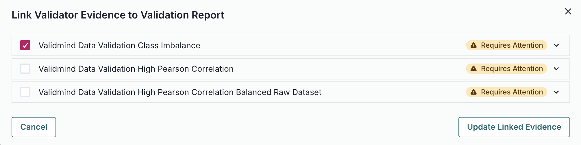
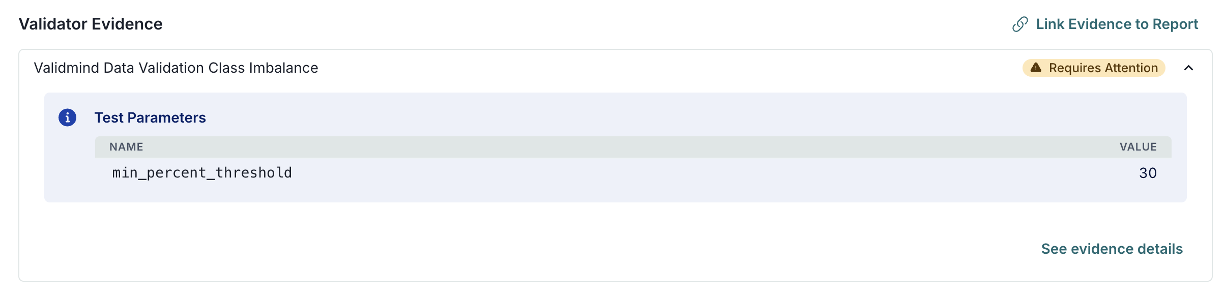
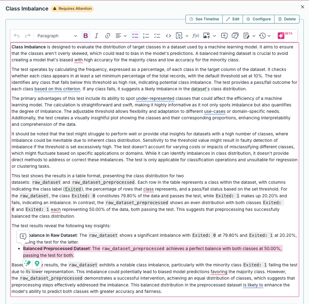
ValidMind for model validation 2 — Start the model validation process

Learn how to use ValidMind for your end-to-end model validation process with our series of four introductory notebooks. In this second notebook, independently verify the data quality tests performed on the dataset used to train the champion model.

You'll learn how to run relevant validation tests with ValidMind, log the results of those tests to the ValidMind Platform, and insert your logged test results as evidence into your validation report. You'll become familiar with the tests available in ValidMind, as well as how to run them. Running tests during model validation is crucial to the effective challenge process, as we want to independently evaluate the evidence and assessments provided by the model development team.

While running our tests in this notebook, we'll focus on:

• Ensuring that data used for training and testing the model is of appropriate data quality
• Ensuring that the raw data has been preprocessed appropriately and that the resulting final datasets reflects this

For a full list of out-of-the-box tests, refer to our Test descriptions or try the interactive Test sandbox.

Learn by doing

Our course tailor-made for validators new to ValidMind combines this series of notebooks with more a more in-depth introduction to the ValidMind Platform — Validator Fundamentals

Prerequisites

In order to independently assess the quality of your datasets with notebook, you'll need to first have:

• Registered a model within the ValidMind Platform and granted yourself access to the model as a validator
• Installed the ValidMind Library in your local environment, allowing you to access all its features

Need help with the above steps?

Refer to the first notebook in this series: 1 — Set up the ValidMind Library for validation

Setting up

Initialize the ValidMind Library

First, let's connect up the ValidMind Library to our model we previously registered in the ValidMind Platform:

1. In a browser, log in to ValidMind.

2. In the left sidebar, navigate to Inventory and select the model you registered for this "ValidMind for model validation" series of notebooks.

3. Go to Getting Started and click Copy snippet to clipboard.

Next, load your model identifier credentials from an .env file or replace the placeholder with your own code snippet:

# Make sure the ValidMind Library is installed

%pip install -q validmind

# Load your model identifier credentials from an `.env` file

%load_ext dotenv
%dotenv .env

# Or replace with your code snippet

import validmind as vm

vm.init(
    # api_host="...",
    # api_key="...",
    # api_secret="...",
    # model="...",
)

Note: you may need to restart the kernel to use updated packages.

2026-01-10 02:35:03,153 - INFO(validmind.api_client): 🎉 Connected to ValidMind!
📊 Model: [ValidMind Academy] Model validation (ID: cmalguc9y02ok199q2db381ib)
📁 Document Type: validation_report

Load the sample dataset

Let's first import the public Bank Customer Churn Prediction dataset from Kaggle, which was used to develop the dummy champion model.

We'll use this dataset to review steps that should have been conducted during the initial development and documentation of the model to ensure that the model was built correctly. By independently performing steps taken by the model development team, we can confirm whether the model was built using appropriate and properly processed data.

In our below example, note that:

• The target column, Exited has a value of 1 when a customer has churned and 0 otherwise.
• The ValidMind Library provides a wrapper to automatically load the dataset as a Pandas DataFrame object. A Pandas Dataframe is a two-dimensional tabular data structure that makes use of rows and columns.

from validmind.datasets.classification import customer_churn as demo_dataset

print(
    f"Loaded demo dataset with: \n\n\t• Target column: '{demo_dataset.target_column}' \n\t• Class labels: {demo_dataset.class_labels}"
)

raw_df = demo_dataset.load_data()
raw_df.head()

Loaded demo dataset with: 

    • Target column: 'Exited' 
    • Class labels: {'0': 'Did not exit', '1': 'Exited'}

	CreditScore	Geography	Gender	Age	Tenure	Balance	NumOfProducts	HasCrCard	IsActiveMember	EstimatedSalary	Exited
0	619	France	Female	42	2	0.00	1	1	1	101348.88	1
1	608	Spain	Female	41	1	83807.86	1	0	1	112542.58	0
2	502	France	Female	42	8	159660.80	3	1	0	113931.57	1
3	699	France	Female	39	1	0.00	2	0	0	93826.63	0
4	850	Spain	Female	43	2	125510.82	1	1	1	79084.10	0

Verifying data quality adjustments

Let's say that thanks to the documentation submitted by the model development team (Learn more ...), we know that the sample dataset was first modified before being used to train the champion model. After performing some data quality assessments on the raw dataset, it was determined that the dataset required rebalancing, and highly correlated features were also removed.

Identify qualitative tests

During model validation, we use the same data processing logic and training procedure to confirm that the model's results can be reproduced independently, so let's start by doing some data quality assessments by running a few individual tests just like the development team did.

Use the vm.tests.list_tests() function introduced by the first notebook in this series in combination with vm.tests.list_tags() and vm.tests.list_tasks() to find which prebuilt tests are relevant for data quality assessment:

• tasks represent the kind of modeling task associated with a test. Here we'll focus on classification tasks.
• tags are free-form descriptions providing more details about the test, for example, what category the test falls into. Here we'll focus on the data_quality tag.

# Get the list of available task types
sorted(vm.tests.list_tasks())

['classification',
 'clustering',
 'data_validation',
 'feature_extraction',
 'monitoring',
 'nlp',
 'regression',
 'residual_analysis',
 'text_classification',
 'text_generation',
 'text_qa',
 'text_summarization',
 'time_series_forecasting',
 'visualization']

# Get the list of available tags
sorted(vm.tests.list_tags())

['AUC',
 'analysis',
 'anomaly_detection',
 'bias_and_fairness',
 'binary_classification',
 'calibration',
 'categorical_data',
 'classification',
 'classification_metrics',
 'clustering',
 'correlation',
 'credit_risk',
 'data_analysis',
 'data_distribution',
 'data_quality',
 'data_validation',
 'descriptive_statistics',
 'dimensionality_reduction',
 'distribution',
 'embeddings',
 'feature_importance',
 'feature_selection',
 'few_shot',
 'forecasting',
 'frequency_analysis',
 'kmeans',
 'linear_regression',
 'llm',
 'logistic_regression',
 'metadata',
 'model_comparison',
 'model_diagnosis',
 'model_explainability',
 'model_interpretation',
 'model_performance',
 'model_predictions',
 'model_selection',
 'model_training',
 'model_validation',
 'multiclass_classification',
 'nlp',
 'normality',
 'numerical_data',
 'outliers',
 'qualitative',
 'rag_performance',
 'ragas',
 'regression',
 'retrieval_performance',
 'scorecard',
 'seasonality',
 'senstivity_analysis',
 'sklearn',
 'stationarity',
 'statistical_test',
 'statistics',
 'statsmodels',
 'tabular_data',
 'text_data',
 'threshold_optimization',
 'time_series_data',
 'unit_root_test',
 'visualization',
 'zero_shot']

You can pass tags and tasks as parameters to the vm.tests.list_tests() function to filter the tests based on the tags and task types.

For example, to find tests related to tabular data quality for classification models, you can call list_tests() like this:

vm.tests.list_tests(task="classification", tags=["tabular_data", "data_quality"])

ID	Name	Description	Has Figure	Has Table	Required Inputs	Params	Tags	Tasks
validmind.data_validation.ClassImbalance	Class Imbalance	Evaluates and quantifies class distribution imbalance in a dataset used by a machine learning model....	True	True	['dataset']	{'min_percent_threshold': {'type': 'int', 'default': 10}}	['tabular_data', 'binary_classification', 'multiclass_classification', 'data_quality']	['classification']
validmind.data_validation.DescriptiveStatistics	Descriptive Statistics	Performs a detailed descriptive statistical analysis of both numerical and categorical data within a model's...	False	True	['dataset']	{}	['tabular_data', 'time_series_data', 'data_quality']	['classification', 'regression']
validmind.data_validation.Duplicates	Duplicates	Tests dataset for duplicate entries, ensuring model reliability via data quality verification....	False	True	['dataset']	{'min_threshold': {'type': '_empty', 'default': 1}}	['tabular_data', 'data_quality', 'text_data']	['classification', 'regression']
validmind.data_validation.HighCardinality	High Cardinality	Assesses the number of unique values in categorical columns to detect high cardinality and potential overfitting....	False	True	['dataset']	{'num_threshold': {'type': 'int', 'default': 100}, 'percent_threshold': {'type': 'float', 'default': 0.1}, 'threshold_type': {'type': 'str', 'default': 'percent'}}	['tabular_data', 'data_quality', 'categorical_data']	['classification', 'regression']
validmind.data_validation.HighPearsonCorrelation	High Pearson Correlation	Identifies highly correlated feature pairs in a dataset suggesting feature redundancy or multicollinearity....	False	True	['dataset']	{'max_threshold': {'type': 'float', 'default': 0.3}, 'top_n_correlations': {'type': 'int', 'default': 10}, 'feature_columns': {'type': 'list', 'default': None}}	['tabular_data', 'data_quality', 'correlation']	['classification', 'regression']
validmind.data_validation.MissingValues	Missing Values	Evaluates dataset quality by ensuring missing value ratio across all features does not exceed a set threshold....	False	True	['dataset']	{'min_threshold': {'type': 'int', 'default': 1}}	['tabular_data', 'data_quality']	['classification', 'regression']
validmind.data_validation.MissingValuesBarPlot	Missing Values Bar Plot	Assesses the percentage and distribution of missing values in the dataset via a bar plot, with emphasis on...	True	False	['dataset']	{'threshold': {'type': 'int', 'default': 80}, 'fig_height': {'type': 'int', 'default': 600}}	['tabular_data', 'data_quality', 'visualization']	['classification', 'regression']
validmind.data_validation.Skewness	Skewness	Evaluates the skewness of numerical data in a dataset to check against a defined threshold, aiming to ensure data...	False	True	['dataset']	{'max_threshold': {'type': '_empty', 'default': 1}}	['data_quality', 'tabular_data']	['classification', 'regression']
validmind.plots.BoxPlot	Box Plot	Generates customizable box plots for numerical features in a dataset with optional grouping using Plotly....	True	False	['dataset']	{'columns': {'type': 'Optional', 'default': None}, 'group_by': {'type': 'Optional', 'default': None}, 'width': {'type': 'int', 'default': 1800}, 'height': {'type': 'int', 'default': 1200}, 'colors': {'type': 'Optional', 'default': None}, 'show_outliers': {'type': 'bool', 'default': True}, 'title_prefix': {'type': 'str', 'default': 'Box Plot of'}}	['tabular_data', 'visualization', 'data_quality']	['classification', 'regression', 'clustering']
validmind.plots.HistogramPlot	Histogram Plot	Generates customizable histogram plots for numerical features in a dataset using Plotly....	True	False	['dataset']	{'columns': {'type': 'Optional', 'default': None}, 'bins': {'type': 'Union', 'default': 30}, 'color': {'type': 'str', 'default': 'steelblue'}, 'opacity': {'type': 'float', 'default': 0.7}, 'show_kde': {'type': 'bool', 'default': True}, 'normalize': {'type': 'bool', 'default': False}, 'log_scale': {'type': 'bool', 'default': False}, 'title_prefix': {'type': 'str', 'default': 'Histogram of'}, 'width': {'type': 'int', 'default': 1200}, 'height': {'type': 'int', 'default': 800}, 'n_cols': {'type': 'int', 'default': 2}, 'vertical_spacing': {'type': 'float', 'default': 0.15}, 'horizontal_spacing': {'type': 'float', 'default': 0.1}}	['tabular_data', 'visualization', 'data_quality']	['classification', 'regression', 'clustering']
validmind.stats.DescriptiveStats	Descriptive Stats	Provides comprehensive descriptive statistics for numerical features in a dataset....	False	True	['dataset']	{'columns': {'type': 'Optional', 'default': None}, 'include_advanced': {'type': 'bool', 'default': True}, 'confidence_level': {'type': 'float', 'default': 0.95}}	['tabular_data', 'statistics', 'data_quality']	['classification', 'regression', 'clustering']

Want to learn more about navigating ValidMind tests?

Refer to our notebook outlining the utilities available for viewing and understanding available ValidMind tests: Explore tests

Initialize the ValidMind datasets

With the individual tests we want to run identified, the next step is to connect your data with a ValidMind Dataset object. This step is always necessary every time you want to connect a dataset to documentation and produce test results through ValidMind, but you only need to do it once per dataset.

Initialize a ValidMind dataset object using the init_dataset function from the ValidMind (vm) module. For this example, we'll pass in the following arguments:

• dataset — The raw dataset that you want to provide as input to tests.
• input_id — A unique identifier that allows tracking what inputs are used when running each individual test.
• target_column — A required argument if tests require access to true values. This is the name of the target column in the dataset.

# vm_raw_dataset is now a VMDataset object that you can pass to any ValidMind test
vm_raw_dataset = vm.init_dataset(
    dataset=raw_df,
    input_id="raw_dataset",
    target_column="Exited",
)

Run data quality tests

Now that we know how to initialize a ValidMind dataset object, we're ready to run some tests!

You run individual tests by calling the run_test function provided by the validmind.tests module. For the examples below, we'll pass in the following arguments:

• test_id — The ID of the test to run, as seen in the ID column when you run list_tests.
• params — A dictionary of parameters for the test. These will override any default_params set in the test definition.

Run tabular data tests

The inputs expected by a test can also be found in the test definition — let's take validmind.data_validation.DescriptiveStatistics as an example.

Note that the output of the describe_test() function below shows that this test expects a dataset as input:

vm.tests.describe_test("validmind.data_validation.DescriptiveStatistics")

▶ Test: Descriptive Statistics ('validmind.data_validation.DescriptiveStatistics')

Descriptive Statistics

Performs a detailed descriptive statistical analysis of both numerical and categorical data within a model's dataset.

Purpose

The purpose of the Descriptive Statistics metric is to provide a comprehensive summary of both numerical and categorical data within a dataset. This involves statistics such as count, mean, standard deviation, minimum and maximum values for numerical data. For categorical data, it calculates the count, number of unique values, most common value and its frequency, and the proportion of the most frequent value relative to the total. The goal is to visualize the overall distribution of the variables in the dataset, aiding in understanding the model's behavior and predicting its performance.

Test Mechanism

The testing mechanism utilizes two in-built functions of pandas dataframes: describe() for numerical fields and value_counts() for categorical fields. The describe() function pulls out several summary statistics, while value_counts() accounts for unique values. The resulting data is formatted into two distinct tables, one for numerical and another for categorical variable summaries. These tables provide a clear summary of the main characteristics of the variables, which can be instrumental in assessing the model's performance.

Signs of High Risk

• Skewed data or significant outliers can represent high risk. For numerical data, this may be reflected via a significant difference between the mean and median (50% percentile).
• For categorical data, a lack of diversity (low count of unique values), or overdominance of a single category (high frequency of the top value) can indicate high risk.

Strengths

• Provides a comprehensive summary of the dataset, shedding light on the distribution and characteristics of the variables under consideration.
• It is a versatile and robust method, applicable to both numerical and categorical data.
• Helps highlight crucial anomalies such as outliers, extreme skewness, or lack of diversity, which are vital in understanding model behavior during testing and validation.

Limitations

• While this metric offers a high-level overview of the data, it may fail to detect subtle correlations or complex patterns.
• Does not offer any insights on the relationship between variables.
• Alone, descriptive statistics cannot be used to infer properties about future unseen data.
• Should be used in conjunction with other statistical tests to provide a comprehensive understanding of the model's data.

Required Inputs: dataset

Parameters:

Parameter	Default Value

How to Run:

Code:

        
import validmind as vm

# inputs dictionary maps your inputs to the expected input names
# keys are the expected input names and values are the actual inputs
# values may be string input_ids or the actual VMDataset or VMModel objects
inputs = {
    "dataset": "my_vm_dataset"
}
params = {}

# to run and view the result of this test, run the following code:
result = vm.tests.run_test(
  "validmind.data_validation.DescriptiveStatistics", inputs=inputs, params=params
)

# To see the result of the test, ensure that you have called `vm.init()` and then run:
result.log()
    

Now, let's run a few tests to assess the quality of the dataset:

result2 = vm.tests.run_test(
    test_id="validmind.data_validation.ClassImbalance",
    inputs={"dataset": vm_raw_dataset},
    params={"min_percent_threshold": 30},
)

❌ Class Imbalance

Class Imbalance is designed to evaluate and quantify the distribution of target classes within a dataset used by a machine learning model, with the primary purpose of identifying whether any class is under-represented to a degree that could introduce bias into the model’s predictions. This test is essential for ensuring that the model is trained on data that reflects a balanced representation of all classes, thereby supporting fair and reliable predictive performance across the entire target space.

The test operates by calculating the frequency of each class in the target column, expressing these frequencies as percentages of the total dataset. It then compares each class’s percentage to a predefined minimum threshold, which in this case is set at 30%. If any class’s proportion falls below this threshold, it is flagged as not meeting the balance criterion. The methodology involves a straightforward count of records for each class, division by the total number of records, and conversion to a percentage. The resulting values typically range from 0% to 100%, where higher values indicate greater representation. A class is considered sufficiently represented if its percentage meets or exceeds the threshold, while lower values signal potential imbalance. The test outputs both a tabular summary and a visual plot, making it easy to interpret the distribution and identify any classes that may be at risk of under-representation.

The primary advantages of this test include its ability to quickly and clearly identify under-represented classes, which is critical for preventing model bias and ensuring robust generalization. The test’s simplicity and speed make it suitable for routine use in model development pipelines, and its quantitative output provides actionable insights for data scientists. The adjustable threshold parameter allows the test to be tailored to specific domain requirements or regulatory standards, enhancing its flexibility. Additionally, the inclusion of a visual plot aids in the rapid assessment of class proportions, supporting both technical and non-technical stakeholders in understanding the dataset’s structure.

It should be noted that the test has several limitations. It may be less informative for datasets with a large number of classes, where some degree of imbalance is expected due to the natural distribution of the data. The choice of threshold is subjective and can influence the test’s sensitivity; setting it too high may result in false positives for imbalance, while setting it too low may overlook meaningful disparities. The test does not account for the varying impact of misclassifying different classes, which can be significant in certain applications. Furthermore, while the test identifies imbalances, it does not provide solutions for addressing them, nor does it consider the downstream effects of imbalance on model performance metrics such as precision, recall, or overall accuracy. Finally, the test is only applicable to classification problems and cannot be used for regression or clustering tasks.

This test shows the results in both tabular and graphical formats. The table titled "Exited Class Imbalance" lists each class in the target variable "Exited," displaying the percentage of rows corresponding to each class and indicating whether the class passes or fails the minimum percentage threshold. Specifically, class 0 comprises 79.80% of the dataset and passes the threshold, while class 1 comprises 20.20% and fails. The accompanying bar plot visually represents these proportions, with the x-axis denoting the class labels (0 and 1) and the y-axis showing the percentage of the dataset each class occupies, ranging from 0 to 1 (or 0% to 100%). The plot clearly illustrates the disparity between the two classes, with class 0 dominating the distribution. The table and plot together provide a comprehensive view of class representation, making it straightforward to identify the imbalance and assess its magnitude relative to the set threshold.

The test results reveal the following key insights:

• Majority Class Dominates Distribution: Class 0 constitutes 79.80% of the dataset, significantly exceeding the minimum threshold and indicating a strong majority presence.
• Minority Class Fails Threshold: Class 1 represents only 20.20% of the dataset, falling below the 30% minimum threshold and failing the test’s criterion for sufficient representation.
• Clear Visual Disparity in Class Proportions: The bar plot visually emphasizes the imbalance, with class 0’s bar substantially higher than that of class 1, reinforcing the quantitative results from the table.
• Binary Target Structure: The dataset contains only two classes, simplifying the interpretation but also highlighting the pronounced imbalance between them.
• Threshold Sensitivity Evident: The choice of a 30% threshold directly impacts the pass/fail outcome, as class 1 would pass at a lower threshold but fails under the current setting.

Based on these results, the dataset exhibits a pronounced class imbalance, with the majority class (class 0) comprising nearly four-fifths of all records and the minority class (class 1) falling short of the minimum representation threshold. The tabular and graphical outputs consistently demonstrate that class 1 is under-represented according to the specified criterion, which may have implications for the model’s ability to accurately predict outcomes for this class. The binary nature of the target variable makes the imbalance particularly evident, and the results underscore the importance of considering class distribution when developing and evaluating classification models. The observed patterns suggest that, under the current threshold, the dataset does not meet the standard for balanced class representation, which could influence the model’s predictive behavior and its performance on minority class instances.

Parameters:

{
  "min_percent_threshold": 30
}
            

Tables

Exited Class Imbalance

Exited	Percentage of Rows (%)	Pass/Fail
0	79.80%	Pass
1	20.20%	Fail

Figures

The output above shows that the class imbalance test did not pass according to the value we set for min_percent_threshold — great, this matches what was reported by the model development team.

To address this issue, we'll re-run the test on some processed data. In this case let's apply a very simple rebalancing technique to the dataset:

import pandas as pd

raw_copy_df = raw_df.sample(frac=1)  # Create a copy of the raw dataset

# Create a balanced dataset with the same number of exited and not exited customers
exited_df = raw_copy_df.loc[raw_copy_df["Exited"] == 1]
not_exited_df = raw_copy_df.loc[raw_copy_df["Exited"] == 0].sample(n=exited_df.shape[0])

balanced_raw_df = pd.concat([exited_df, not_exited_df])
balanced_raw_df = balanced_raw_df.sample(frac=1, random_state=42)

With this new balanced dataset, you can re-run the individual test to see if it now passes the class imbalance test requirement.

As this is technically a different dataset, remember to first initialize a new ValidMind Dataset object to pass in as input as required by run_test():

# Register new data and now 'balanced_raw_dataset' is the new dataset object of interest
vm_balanced_raw_dataset = vm.init_dataset(
    dataset=balanced_raw_df,
    input_id="balanced_raw_dataset",
    target_column="Exited",
)

# Pass the initialized `balanced_raw_dataset` as input into the test run
result = vm.tests.run_test(
    test_id="validmind.data_validation.ClassImbalance",
    inputs={"dataset": vm_balanced_raw_dataset},
    params={"min_percent_threshold": 30},
)

✅ Class Imbalance

Class Imbalance is designed to evaluate and quantify the distribution of target classes within a dataset used by a machine learning model, with the primary purpose of identifying whether any class is under-represented to a degree that could introduce bias into the model’s predictions. By systematically assessing the proportion of each class, the test aims to ensure that the dataset is sufficiently balanced to support robust and fair model training and evaluation.

The test operates by calculating the frequency of each class in the target column, expressing these frequencies as percentages of the total dataset. It then compares each class’s percentage to a predefined minimum threshold, which in this case is set at 30%. If any class falls below this threshold, it is flagged as potentially imbalanced, and the test marks it as a fail for that class. The methodology is straightforward: it requires the target column as input and counts the number of occurrences for each unique class label. These counts are divided by the total number of records to yield a percentage for each class, which is then compared to the threshold. The output includes both a pass/fail indicator for each class and a visual representation of the class proportions. The percentages range from 0% to 100%, where higher values indicate greater representation. A class percentage below the threshold is generally interpreted as a sign of potential imbalance, which could affect model performance, while percentages above the threshold suggest adequate representation.

The primary advantages of this test include its ability to quickly and clearly identify under-represented classes that may impact model performance, especially in scenarios where class balance is critical for predictive accuracy and fairness. The test’s simplicity and speed make it suitable for routine data quality checks, and its quantitative output provides clear, actionable information. The adjustable threshold allows users to tailor the test to specific domain requirements, making it flexible for a variety of applications. The inclusion of a visual plot enhances interpretability, allowing stakeholders to easily grasp the class distribution at a glance. This is particularly useful in regulated environments or high-stakes applications where transparency and explainability are essential.

It should be noted that the test has several limitations. It may be less informative for datasets with a large number of classes, where some degree of imbalance is expected or unavoidable. The results are sensitive to the chosen threshold; setting this value too high may result in false positives for imbalance, while setting it too low may overlook meaningful disparities. The test does not account for the varying costs or consequences of misclassifying different classes, which can be significant in certain domains. Additionally, while the test can identify the presence and degree of imbalance, it does not provide guidance or methods for addressing these issues. Its applicability is limited to classification tasks and does not extend to regression or clustering problems. Finally, the test’s pass/fail outcome is based solely on class proportions and does not consider other aspects of data quality or model performance.

This test shows the results in both tabular and graphical formats. The table titled "Exited Class Imbalance" lists each class in the target variable ("Exited"), the percentage of rows corresponding to each class, and a pass/fail indicator based on the 30% minimum threshold. In this case, there are two classes: 0 and 1, each representing 50.00% of the dataset, and both are marked as "Pass." The accompanying bar plot visually displays the proportion of each class, with the x-axis representing the class labels (0 and 1) and the y-axis showing the percentage of the dataset that each class comprises. Both bars reach the 0.5 mark, corresponding to 50%, and are visually identical in height, indicating perfect balance between the two classes. The scale of the plot ranges from 0 to 0.5 (or 0% to 50%), and the uniformity of the bars confirms the numerical results from the table. There are no classes below the threshold, and no notable deviations or outliers are present. The results are straightforward to interpret: both classes are equally represented, and the dataset passes the class imbalance test for the specified threshold.

The test results reveal the following key insights:

• Both classes meet the minimum representation threshold: Each class in the "Exited" target variable constitutes exactly 50.00% of the dataset, which is well above the 30% minimum threshold set for this test.
• Perfectly balanced class distribution: The dataset exhibits an even split between the two classes, as shown by both the tabular data and the bar plot, with no observable skew or dominance by either class.
• Consistent pass outcome across all classes: Both classes are marked as "Pass" in the results table, indicating that neither class is under-represented according to the test criteria.
• Visual confirmation of numerical results: The bar plot provides a clear visual affirmation of the tabular data, with both bars reaching the same height and no visual indication of imbalance or irregularity.
• No evidence of class imbalance risk: There are no classes flagged as failing the threshold, and the distribution is stable across the entire dataset, suggesting a low risk of model bias due to class imbalance.

Based on these results, the dataset used for the "Exited" target variable demonstrates a perfectly balanced class distribution, with both classes equally represented at 50.00%. This balance is confirmed by both the numerical table and the visual plot, and both classes comfortably exceed the 30% minimum threshold required by the test. The absence of any class below the threshold indicates that the risk of model bias due to class imbalance is minimal for this dataset. The results suggest that the model trained on this data is unlikely to exhibit preferential performance for one class over the other solely due to class distribution. The uniformity observed in both the tabular and graphical outputs provides strong evidence of data stability and consistency, supporting the reliability of subsequent model training and evaluation processes. The test’s clear pass outcome for all classes further reinforces the conclusion that the dataset is well-suited for classification tasks without the need for additional balancing interventions.

Parameters:

{
  "min_percent_threshold": 30
}
            

Tables

Exited Class Imbalance

Exited	Percentage of Rows (%)	Pass/Fail
0	50.00%	Pass
1	50.00%	Pass

Figures

Remove highly correlated features

Next, let's also remove highly correlated features from our dataset as outlined by the development team. Removing highly correlated features helps make the model simpler, more stable, and easier to understand.

You can utilize the output from a ValidMind test for further use — in this below example, to retrieve the list of features with the highest correlation coefficients and use them to reduce the final list of features for modeling.

First, we'll run validmind.data_validation.HighPearsonCorrelation with the balanced_raw_dataset we initialized previously as input as is for comparison with later runs:

corr_result = vm.tests.run_test(
    test_id="validmind.data_validation.HighPearsonCorrelation",
    params={"max_threshold": 0.3},
    inputs={"dataset": vm_balanced_raw_dataset},
)

❌ High Pearson Correlation

High Pearson Correlation is designed to identify pairs of features within a dataset that exhibit strong linear relationships, with the primary purpose of detecting potential feature redundancy or multicollinearity. This is crucial for ensuring that the predictive model remains interpretable and robust, as high correlations between features can obscure the true impact of individual variables and may lead to overfitting or instability in model estimates.

The test operates by calculating the Pearson correlation coefficient for every possible pair of features in the dataset. The Pearson correlation coefficient is a statistical measure that quantifies the strength and direction of a linear relationship between two continuous variables, producing values that range from -1 to 1. A value of 1 indicates a perfect positive linear relationship, -1 indicates a perfect negative linear relationship, and 0 indicates no linear relationship. The test systematically computes these coefficients for all feature pairs, removes self-correlations and duplicate pairs, and then compares the absolute value of each coefficient to a predefined threshold, which in this case is set at 0.3. Any pair with an absolute correlation exceeding this threshold is flagged as a potential risk for multicollinearity. The test then presents the top n strongest correlations, regardless of whether they pass or fail the threshold, providing a transparent view of the most significant linear relationships in the data.

The primary advantages of this test include its efficiency and transparency in surfacing linear dependencies between features, which is particularly valuable during the early stages of model development and risk assessment. By highlighting pairs of variables with strong linear associations, the test enables practitioners to quickly identify and address potential sources of redundancy or instability in the model. This can help prevent issues such as inflated variance in model coefficients, reduced interpretability, and overfitting. The clear tabular output, which lists feature pairs, their correlation coefficients, and pass/fail status, supports straightforward communication of results to both technical and non-technical stakeholders, facilitating informed decision-making regarding feature selection and engineering.

It should be noted that the test is limited to detecting only linear relationships, as the Pearson correlation coefficient does not capture nonlinear dependencies that may exist between features. Additionally, the metric is sensitive to outliers, which can disproportionately influence the calculated coefficients and potentially exaggerate or mask true relationships. The test also focuses exclusively on pairwise relationships, meaning it may not detect more complex forms of multicollinearity involving three or more variables. High correlation coefficients, particularly those exceeding the threshold, are indicative of potential risk, as they suggest that the associated features may be redundant or could introduce instability into the model. However, the presence of high correlations does not automatically imply a problem; further analysis is often required to determine the practical impact on model performance.

This test shows its results in a tabular format, where each row represents a unique pair of features from the dataset. The columns include the feature pair, the calculated Pearson correlation coefficient (rounded to four decimal places), and a pass/fail status based on whether the absolute value of the coefficient exceeds the threshold of 0.3. The coefficients range from approximately -0.21 to 0.34, with both positive and negative values indicating the direction of the linear relationship. The table is sorted by the absolute value of the coefficient, with the strongest correlations listed first. Notably, only one feature pair, (Age, Exited), exceeds the threshold and is marked as "Fail," while all other pairs are below the threshold and marked as "Pass." The table provides a clear and concise overview of the most significant linear relationships in the dataset, allowing users to quickly assess the extent and nature of potential multicollinearity.

The test results reveal the following key insights:

• Single Feature Pair Exceeds Correlation Threshold: Only the pair (Age, Exited) has a Pearson correlation coefficient of 0.3405, surpassing the threshold of 0.3 and resulting in a "Fail" status, indicating a moderate positive linear relationship between these features.
• All Other Feature Pairs Remain Below Threshold: The remaining nine feature pairs have coefficients ranging from -0.2064 to 0.1507, all of which are below the 0.3 threshold and are marked as "Pass," suggesting limited risk of multicollinearity among these pairs.
• Distribution of Correlation Coefficients Is Centered Near Zero: Most coefficients are relatively close to zero, with both positive and negative values, indicating that the majority of feature pairs do not exhibit strong linear relationships.
• Negative and Positive Relationships Are Both Present: The table includes both positive and negative coefficients, such as (IsActiveMember, Exited) at -0.2064 and (Balance, Exited) at 0.1507, reflecting a mix of direct and inverse linear associations.
• No Evidence of Widespread Multicollinearity: The limited number of pairs exceeding the threshold and the generally low magnitude of coefficients suggest that the dataset does not exhibit pervasive multicollinearity among its features.

Based on these results, the dataset demonstrates a generally low level of linear association between most feature pairs, with only one pair, (Age, Exited), exhibiting a moderate positive correlation that exceeds the predefined threshold. This observation indicates that, aside from this specific relationship, the features are largely independent in terms of linear association, reducing the likelihood of multicollinearity adversely affecting model interpretability or stability. The presence of both positive and negative coefficients further suggests a balanced distribution of relationships, with no single direction dominating the dataset. The clear separation between the one "Fail" and the remaining "Pass" pairs provides a straightforward view of where potential redundancy may exist, while the overall low magnitude of coefficients supports the conclusion that the feature set is well-structured with respect to linear dependencies. This pattern of results is consistent with a dataset that is suitable for modeling without significant risk of linear redundancy, aside from the noted (Age, Exited) relationship, which may warrant further examination depending on the modeling context.

Parameters:

{
  "max_threshold": 0.3
}
            

Tables

Columns	Coefficient	Pass/Fail
(Age, Exited)	0.3405	Fail
(IsActiveMember, Exited)	-0.2064	Pass
(Balance, NumOfProducts)	-0.1730	Pass
(Balance, Exited)	0.1507	Pass
(NumOfProducts, Exited)	-0.0558	Pass
(Age, Balance)	0.0548	Pass
(Tenure, Exited)	-0.0516	Pass
(Age, NumOfProducts)	-0.0457	Pass
(NumOfProducts, IsActiveMember)	0.0433	Pass
(HasCrCard, IsActiveMember)	-0.0412	Pass

The output above shows that the test did not pass according to the value we set for max_threshold — as reported and expected.

corr_result is an object of type TestResult. We can inspect the result object to see what the test has produced:

print(type(corr_result))
print("Result ID: ", corr_result.result_id)
print("Params: ", corr_result.params)
print("Passed: ", corr_result.passed)
print("Tables: ", corr_result.tables)

<class 'validmind.vm_models.result.result.TestResult'>
Result ID:  validmind.data_validation.HighPearsonCorrelation
Params:  {'max_threshold': 0.3}
Passed:  False
Tables:  [ResultTable]

Let's remove the highly correlated features and create a new VM dataset object.

We'll begin by checking out the table in the result and extracting a list of features that failed the test:

# Extract table from `corr_result.tables`
features_df = corr_result.tables[0].data
features_df

	Columns	Coefficient	Pass/Fail
0	(Age, Exited)	0.3405	Fail
1	(IsActiveMember, Exited)	-0.2064	Pass
2	(Balance, NumOfProducts)	-0.1730	Pass
3	(Balance, Exited)	0.1507	Pass
4	(NumOfProducts, Exited)	-0.0558	Pass
5	(Age, Balance)	0.0548	Pass
6	(Tenure, Exited)	-0.0516	Pass
7	(Age, NumOfProducts)	-0.0457	Pass
8	(NumOfProducts, IsActiveMember)	0.0433	Pass
9	(HasCrCard, IsActiveMember)	-0.0412	Pass

# Extract list of features that failed the test
high_correlation_features = features_df[features_df["Pass/Fail"] == "Fail"]["Columns"].tolist()
high_correlation_features

['(Age, Exited)']

Next, extract the feature names from the list of strings (example: (Age, Exited) > Age):

high_correlation_features = [feature.split(",")[0].strip("()") for feature in high_correlation_features]
high_correlation_features

['Age']

Now, it's time to re-initialize the dataset with the highly correlated features removed.

Note the use of a different input_id. This allows tracking the inputs used when running each individual test.

# Remove the highly correlated features from the dataset
balanced_raw_no_age_df = balanced_raw_df.drop(columns=high_correlation_features)

# Re-initialize the dataset object
vm_raw_dataset_preprocessed = vm.init_dataset(
    dataset=balanced_raw_no_age_df,
    input_id="raw_dataset_preprocessed",
    target_column="Exited",
)

Re-running the test with the reduced feature set should pass the test:

corr_result = vm.tests.run_test(
    test_id="validmind.data_validation.HighPearsonCorrelation",
    params={"max_threshold": 0.3},
    inputs={"dataset": vm_raw_dataset_preprocessed},
)

✅ High Pearson Correlation

High Pearson Correlation is designed to identify pairs of features within a dataset that exhibit strong linear relationships, with the primary purpose of detecting potential feature redundancy or multicollinearity. This is crucial for ensuring that the predictive model remains interpretable and robust, as highly correlated features can obscure the true impact of individual variables and may lead to overfitting or instability in model coefficients.

The test operates by calculating the Pearson correlation coefficient for every possible pair of features in the dataset. The Pearson correlation coefficient is a statistical measure that quantifies the strength and direction of a linear relationship between two continuous variables, producing a value between -1 and 1. A value close to 1 indicates a strong positive linear relationship, while a value close to -1 indicates a strong negative linear relationship; values near 0 suggest little to no linear association. The test systematically computes these coefficients for all feature pairs, removes self-correlations and duplicate pairs, and then compares the absolute value of each coefficient to a predefined threshold (in this case, 0.3). If any pair exceeds this threshold, it is flagged as potentially problematic. The test then returns the top n pairs with the highest absolute correlations, along with their coefficients and a Pass or Fail status based on the threshold. This approach provides a transparent and quantitative assessment of linear dependencies among features, which is essential for diagnosing multicollinearity risks in model development.

The primary advantages of this test include its efficiency and clarity in surfacing linear relationships between features, which can be critical for both model performance and interpretability. By providing a ranked list of the strongest correlations, the test enables practitioners to quickly pinpoint which feature pairs may warrant further investigation or remedial action, such as feature selection or transformation. The output is straightforward, presenting both the magnitude and direction of each correlation, as well as a clear Pass or Fail status relative to the chosen threshold. This transparency supports effective communication among data scientists, model risk managers, and stakeholders, and facilitates early detection of multicollinearity, which can otherwise compromise the stability and reliability of model estimates. The test is particularly useful in the initial stages of model development, where understanding the structure and relationships within the data is paramount.

It should be noted that the test is limited to detecting linear relationships and does not capture more complex, nonlinear dependencies that may exist between features. The Pearson correlation coefficient is also sensitive to outliers, which can distort the true strength of association between variables. Additionally, the test only evaluates pairwise relationships and may miss higher-order interactions involving three or more features. Interpretation of the results requires caution, as a high correlation does not necessarily imply causation or redundancy in all modeling contexts. The presence of coefficients exceeding the threshold is a sign of potential risk, as it may indicate multicollinearity or feature redundancy, but further analysis is often needed to determine the practical impact on model performance and interpretability.

This test shows its results in the form of a table, where each row represents a unique pair of features from the dataset. The table includes columns for the feature pair, the Pearson correlation coefficient, and a Pass or Fail status based on whether the absolute value of the coefficient exceeds the threshold of 0.3. The coefficients are presented as decimal values ranging from -1 to 1, with negative values indicating inverse relationships and positive values indicating direct relationships. All reported coefficients in this output are below the threshold, and each pair is marked as Pass. The strongest observed correlation is between IsActiveMember and Exited, with a coefficient of -0.2064, indicating a moderate negative linear relationship. Other notable pairs include Balance and NumOfProducts (-0.173), and Balance and Exited (0.1507). The remaining pairs exhibit weaker correlations, with coefficients ranging from approximately -0.0558 to -0.0309. The table is sorted by the absolute value of the correlation coefficient, allowing for quick identification of the most strongly related feature pairs. No pair exceeds the threshold, and the range of coefficients suggests that the dataset does not exhibit high linear dependencies among its features.

The test results reveal the following key insights:

• No Feature Pair Exceeds Correlation Threshold: All reported feature pairs have absolute Pearson correlation coefficients below the threshold of 0.3, indicating no strong linear relationships that would trigger a Fail status.
• Moderate Negative Correlation Between IsActiveMember and Exited: The strongest observed relationship is a moderate negative correlation of -0.2064 between IsActiveMember and Exited, suggesting that active members are somewhat less likely to have exited.
• Balance Shows Weak Associations with Multiple Features: Balance is involved in several of the top correlations, including with NumOfProducts (-0.173) and Exited (0.1507), but all remain below the threshold, indicating only weak to moderate associations.
• Low Correlations Across Remaining Feature Pairs: The rest of the feature pairs, such as NumOfProducts and Exited (-0.0558), Tenure and Exited (-0.0516), and CreditScore and EstimatedSalary (-0.0335), display low correlation coefficients, suggesting minimal linear dependency.
• Consistent Pass Status Across All Pairs: Every feature pair in the output is marked as Pass, reflecting the absence of any pairwise linear relationships that would be considered high risk under the defined threshold.

Based on these results, the dataset demonstrates a generally low level of linear association among its features, as evidenced by the absence of any pairwise Pearson correlation coefficients exceeding the 0.3 threshold. The most notable relationship, between IsActiveMember and Exited, is moderate but does not approach the level that would indicate a risk of multicollinearity or feature redundancy. The distribution of coefficients, with most values clustered well below the threshold, suggests that the features are largely independent in terms of linear relationships, which supports the interpretability and stability of subsequent modeling efforts. The consistent Pass status across all pairs further reinforces the observation that the dataset does not exhibit problematic linear dependencies that could undermine model performance or complicate interpretation. These results provide a clear quantitative characterization of the feature space, indicating that, from a linear correlation perspective, the dataset is well-structured for use in predictive modeling without immediate risk of multicollinearity.

Parameters:

{
  "max_threshold": 0.3
}
            

Tables

Columns	Coefficient	Pass/Fail
(IsActiveMember, Exited)	-0.2064	Pass
(Balance, NumOfProducts)	-0.1730	Pass
(Balance, Exited)	0.1507	Pass
(NumOfProducts, Exited)	-0.0558	Pass
(Tenure, Exited)	-0.0516	Pass
(NumOfProducts, IsActiveMember)	0.0433	Pass
(HasCrCard, IsActiveMember)	-0.0412	Pass
(CreditScore, Exited)	-0.0412	Pass
(CreditScore, EstimatedSalary)	-0.0335	Pass
(Balance, HasCrCard)	-0.0309	Pass

You can also plot the correlation matrix to visualize the new correlation between features:

corr_result = vm.tests.run_test(
    test_id="validmind.data_validation.PearsonCorrelationMatrix",
    inputs={"dataset": vm_raw_dataset_preprocessed},
)

Pearson Correlation Matrix

Pearson Correlation Matrix is designed to evaluate the extent of linear dependency between all pairs of numerical variables in a dataset. Its primary purpose is to identify potential redundancy among variables by quantifying the strength and direction of their linear relationships, thereby supporting dimensionality reduction and improving model interpretability.

The test operates by calculating the Pearson correlation coefficient for every pair of numerical variables in the dataset. This coefficient measures the degree to which two variables move together in a linear fashion, with values ranging from -1 to 1. A value of 1 indicates a perfect positive linear relationship, -1 indicates a perfect negative linear relationship, and 0 indicates no linear relationship. The test compiles these coefficients into a correlation matrix, which is then visualized as a heat map. The heat map uses color gradients to represent the magnitude and direction of each correlation, with a specific highlight (white) for coefficients whose absolute value exceeds 0.7, signaling a high degree of correlation. This approach allows for rapid identification of variable pairs that may be redundant or highly interdependent, which is particularly useful for feature selection and multicollinearity assessment in modeling workflows.

The primary advantages of this test include its ability to provide a clear, quantitative assessment of linear relationships between variables, which is essential for detecting redundancy and potential multicollinearity in datasets. The heat map visualization makes it accessible to a broad audience, including those less familiar with statistical matrices, by offering an intuitive overview of the correlation structure. This test is especially valuable in scenarios where model simplicity and interpretability are priorities, as it helps to pinpoint variables that may be safely removed or combined without significant loss of information. Additionally, by identifying highly correlated variables, the test supports more robust model development and can help prevent overfitting due to redundant features.

It should be noted that the Pearson Correlation Matrix is limited to detecting linear relationships and may not capture more complex, non-linear dependencies between variables. As a result, important associations could be overlooked if they do not manifest as linear correlations. The test also does not measure the strength of causal influence, only the degree of co-movement. The threshold of 0.7 for highlighting high correlations is somewhat arbitrary and may not be appropriate for all datasets or modeling contexts. Furthermore, a large number of highly correlated variables can indicate redundancy and increase the risk of overfitting, but the test does not provide guidance on which variables to remove or retain. Interpretation challenges may arise if users conflate correlation with causation or overlook the potential for spurious correlations in large datasets.

This test shows a heat map representation of the Pearson correlation matrix for the dataset’s numerical variables. Each cell in the matrix corresponds to the correlation coefficient between a pair of variables, with the variable names listed along both the horizontal and vertical axes. The color scale ranges from deep blue (indicating strong positive correlation) through white (no correlation) to deep red (strong negative correlation), as shown by the color bar on the right. The diagonal cells, which represent the correlation of each variable with itself, are always 1 and are shown in the darkest blue. The off-diagonal cells display the pairwise correlations, with numerical values provided for each cell. Notably, none of the off-diagonal coefficients exceed the ±0.7 threshold, so no cells are highlighted in white for high correlation. The majority of the coefficients are close to zero, indicating weak or negligible linear relationships between most variable pairs. The largest observed absolute correlation is -0.21 between "Exited" and "IsActiveMember," and 0.15 between "Exited" and "Balance," both of which are well below the high-correlation threshold. The heat map provides a comprehensive visual summary, making it easy to identify both the absence of strong linear dependencies and the general independence of the variables.

The test results reveal the following key insights:

• No High Linear Correlations Detected: All off-diagonal correlation coefficients fall well below the ±0.7 threshold, indicating an absence of strong linear relationships between any pair of variables.
• Predominance of Weak Correlations: Most correlation values are clustered near zero, with the majority ranging between -0.21 and 0.15, suggesting that the variables are largely independent in a linear sense.
• Notable Variable Pairs with Moderate Correlation: The strongest observed correlations are -0.21 between "Exited" and "IsActiveMember" and 0.15 between "Exited" and "Balance," but these remain weak and unlikely to indicate redundancy.
• Symmetry and Consistency Across the Matrix: The matrix is symmetric, as expected, and the diagonal values are all 1, confirming the correct computation and representation of the correlation structure.
• Absence of Redundant Features: The lack of high correlations suggests that each variable contributes unique information, with minimal risk of redundancy or multicollinearity.

Based on these results, the dataset exhibits a low degree of linear dependency among its numerical variables, as evidenced by the uniformly weak Pearson correlation coefficients. The absence of any coefficients exceeding the ±0.7 threshold indicates that no pairs of variables are strongly linearly related, minimizing the risk of redundancy and multicollinearity in subsequent modeling. This pattern suggests that each variable is likely to provide distinct information to the model, supporting robust feature selection and reducing the likelihood of overfitting due to correlated predictors. The heat map visualization confirms the general independence of the variables, with no clusters or groupings of high correlation. These characteristics collectively imply that the dataset is well-suited for modeling tasks that assume variable independence, and that dimensionality reduction based solely on linear correlation is not warranted. The observed weak correlations also suggest that any further investigation into variable relationships should consider potential non-linear dependencies, as linear analysis alone does not reveal any significant associations.

Figures

Documenting test results

Now that we've done some analysis on two different datasets, we can use ValidMind to easily document why certain things were done to our raw data with testing to support it. Every test result returned by the run_test() function has a .log() method that can be used to send the test results to the ValidMind Platform.

When logging validation test results to the platform, you'll need to manually add those results to the desired section of the validation report. To demonstrate how to add test results to your validation report, we'll log our data quality tests and insert the results via the ValidMind Platform.

Configure and run comparison tests

Below, we'll perform comparison tests between the original raw dataset (raw_dataset) and the final preprocessed (raw_dataset_preprocessed) dataset, again logging the results to the ValidMind Platform.

We can specify all the tests we'd ike to run in a dictionary called test_config, and we'll pass in the following arguments for each test:

• params: Individual test parameters.
• input_grid: Individual test inputs to compare. In this case, we'll input our two datasets for comparison.

Note here that the input_grid expects the input_id of the dataset as the value rather than the variable name we specified:

# Individual test config with inputs specified
test_config = {
    "validmind.data_validation.ClassImbalance": {
        "input_grid": {"dataset": ["raw_dataset", "raw_dataset_preprocessed"]},
        "params": {"min_percent_threshold": 30}
    },
    "validmind.data_validation.HighPearsonCorrelation": {
        "input_grid": {"dataset": ["raw_dataset", "raw_dataset_preprocessed"]},
        "params": {"max_threshold": 0.3}
    },
}

Then batch run and log our tests in test_config:

for t in test_config:
    print(t)
    try:
        # Check if test has input_grid
        if 'input_grid' in test_config[t]:
            # For tests with input_grid, pass the input_grid configuration
            if 'params' in test_config[t]:
                vm.tests.run_test(t, input_grid=test_config[t]['input_grid'], params=test_config[t]['params']).log()
            else:
                vm.tests.run_test(t, input_grid=test_config[t]['input_grid']).log()
        else:
            # Original logic for regular inputs
            if 'params' in test_config[t]:
                vm.tests.run_test(t, inputs=test_config[t]['inputs'], params=test_config[t]['params']).log()
            else:
                vm.tests.run_test(t, inputs=test_config[t]['inputs']).log()
    except Exception as e:
        print(f"Error running test {t}: {str(e)}")

validmind.data_validation.ClassImbalance

❌ Class Imbalance

Class Imbalance is designed to evaluate and quantify the distribution of target classes within a dataset used by a machine learning model, with the primary purpose of identifying whether any class is under-represented to a degree that could introduce bias into the model’s predictions. By systematically assessing the proportion of each class, the test aims to ensure that the dataset supports the development of models that are not disproportionately influenced by the majority class, thereby promoting fairness and predictive reliability.

The test operates by calculating the frequency of each class in the target column, expressing these frequencies as percentages of the total dataset. It then compares each class’s percentage to a configurable minimum threshold, which in this case is set at 30%. If any class falls below this threshold, it is flagged as not meeting the balance criterion. The test outputs both tabular and graphical representations: the table lists each class, its percentage of the dataset, and a pass/fail status, while the bar plot visually displays the proportion of each class. The metric used—percentage of rows per class—ranges from 0% to 100%, with higher values indicating greater representation. A class is considered adequately represented if its percentage meets or exceeds the threshold; otherwise, it is considered under-represented, which may signal a risk of model bias or reduced generalizability.

The primary advantages of this test include its ability to quickly and transparently highlight class distribution patterns that could impact model performance. The straightforward calculation and clear visualizations make it accessible to a wide range of stakeholders, from data scientists to business analysts. The test’s flexibility, enabled by the adjustable threshold, allows it to be tailored to different domains and risk tolerances. By quantifying the degree of imbalance, it provides actionable insights that can inform data preprocessing or model selection strategies. The visual output further enhances interpretability, making it easy to communicate the state of class balance to both technical and non-technical audiences.

It should be noted that the test has several limitations. It may be less informative for datasets with a large number of classes, where some degree of imbalance is expected due to the natural distribution of the data. The results are sensitive to the chosen threshold; setting this value too high may result in false positives for imbalance, while too low a threshold could overlook meaningful disparities. The test does not account for the varying costs or consequences of misclassifying different classes, which can be critical in certain applications. Additionally, while the test identifies imbalances, it does not provide direct solutions or corrective actions. Its applicability is limited to classification tasks and does not extend to regression or clustering problems. High-risk signs, such as any class falling below the threshold, should be interpreted in the context of the specific modeling objectives and domain requirements.

This test shows the results in both tabular and graphical formats, providing a comprehensive view of class distribution before and after preprocessing. The tables present the dataset name, class label (Exited), percentage of rows for each class, and a pass/fail status based on the 30% threshold. For the raw dataset, class 0 constitutes 79.80% of the data and passes the threshold, while class 1 makes up 20.20% and fails. In the preprocessed dataset, both classes are perfectly balanced at 50.00%, each passing the threshold. The accompanying bar plots visually reinforce these results: the first plot for the raw dataset shows a pronounced imbalance, with class 0 dominating, while the second plot for the preprocessed dataset displays equal bar heights, indicating perfect balance. The y-axis in both plots represents the percentage of the dataset, ranging from 0 to 1 (or 0% to 100%), and the x-axis denotes the class labels. These visualizations make it easy to identify the extent and direction of any imbalance, as well as the impact of preprocessing steps on class distribution.

The test results reveal the following key insights:

• Raw dataset exhibits significant class imbalance: In the raw dataset, class 0 accounts for 79.80% of the records, while class 1 represents only 20.20%, resulting in a fail status for class 1 under the 30% threshold.
• Preprocessing achieves perfect class balance: After preprocessing, both classes in the dataset are equally represented at 50.00%, and both pass the minimum threshold, indicating successful mitigation of imbalance.
• Visualizations clearly differentiate class distributions: The bar plots provide an immediate visual comparison, with the raw dataset showing a stark disparity and the preprocessed dataset displaying equal representation.
• Threshold sensitivity is evident in pass/fail outcomes: The choice of a 30% threshold directly influences the pass/fail status, highlighting the importance of threshold selection in interpreting class balance.
• Preprocessing impact is quantifiable and transparent: The side-by-side comparison of raw and preprocessed datasets demonstrates the effectiveness of preprocessing interventions in addressing class imbalance.

Based on these results, the analysis demonstrates that the raw dataset initially contains a pronounced class imbalance, with the majority class (Exited = 0) far exceeding the minority class (Exited = 1) in representation, as evidenced by both the tabular percentages and the visual disparity in the bar plot. This imbalance is significant enough that the minority class fails the 30% minimum threshold, indicating a potential risk for model bias if left unaddressed. However, after preprocessing, the class distribution is adjusted to achieve perfect balance, with both classes comprising exactly half of the dataset and passing the threshold. The visualizations corroborate these quantitative results, making the shift from imbalance to balance immediately apparent. The test thus provides clear, objective evidence of the initial class distribution and the effectiveness of preprocessing steps in achieving a balanced dataset, which is critical for supporting unbiased model development and reliable predictive performance.

Parameters:

{
  "min_percent_threshold": 30
}
            

Tables

dataset	Exited	Percentage of Rows (%)	Pass/Fail
raw_dataset	0	79.80%	Pass
raw_dataset	1	20.20%	Fail
raw_dataset_preprocessed	0	50.00%	Pass
raw_dataset_preprocessed	1	50.00%	Pass

Figures

2026-01-10 02:37:30,664 - INFO(validmind.vm_models.result.result): Test driven block with result_id validmind.data_validation.ClassImbalance does not exist in model's document

validmind.data_validation.HighPearsonCorrelation

❌ High Pearson Correlation

High Pearson Correlation is designed to identify pairs of features within a dataset that exhibit strong linear relationships, with the primary purpose of detecting potential feature redundancy or multicollinearity. This is crucial for ensuring that the predictive model remains interpretable and robust, as high correlations between features can obscure the unique contribution of each variable and may lead to instability in model estimates.

The test operates by calculating the Pearson correlation coefficient for every possible pair of features in the dataset. The Pearson correlation coefficient quantifies the strength and direction of the linear relationship between two continuous variables, producing a value that ranges from -1 to 1. A value close to 1 indicates a strong positive linear relationship, while a value close to -1 indicates a strong negative linear relationship; values near 0 suggest little to no linear association. The test systematically excludes self-correlations and duplicate pairs, then sorts the results by the absolute value of the coefficient. Each pair is evaluated against a predefined threshold (in this case, 0.3), and a Pass or Fail status is assigned depending on whether the absolute correlation exceeds this threshold. The test outputs the top n strongest correlations, providing a clear view of the most significant linear relationships present in the data.

The primary advantages of this test include its efficiency and transparency in surfacing linear dependencies between features, which is particularly valuable during the early stages of model development and risk assessment. By highlighting pairs of features with high correlation, the test enables practitioners to quickly identify and address potential sources of multicollinearity, which can otherwise compromise model interpretability and predictive stability. The clear tabular output, which lists feature pairs, correlation coefficients, and Pass/Fail status, supports straightforward communication of results to both technical and non-technical stakeholders. This makes the test especially useful for regulatory documentation and for guiding feature selection or engineering decisions in environments where model transparency and reliability are paramount.

It should be noted that the test is limited to detecting linear relationships and does not capture more complex, nonlinear dependencies that may exist between features. The Pearson correlation coefficient is also sensitive to outliers, which can distort the measured strength of association and potentially lead to misleading interpretations. Additionally, the test only evaluates pairwise relationships, so it may not identify multicollinearity that arises from interactions among three or more variables. High correlation coefficients, particularly those exceeding the threshold, are indicative of potential risk, as they may signal redundancy or instability in the model, but the test does not provide direct guidance on how to address these situations or on the impact of such correlations on downstream model performance.

This test shows its results in the form of a table, where each row represents a unique pair of features from either the raw or preprocessed dataset. The columns include the dataset name, the feature pair, the Pearson correlation coefficient (rounded to four decimal places), and a Pass/Fail status based on whether the absolute value of the coefficient exceeds the threshold of 0.3. The coefficients range from approximately -0.30 to 0.28, with negative values indicating inverse relationships and positive values indicating direct relationships. The Pass/Fail column provides a quick reference for identifying pairs that surpass the risk threshold. Notably, only one pair—(Balance, NumOfProducts) in the raw dataset—exceeds the threshold, with a coefficient of -0.3045 and a Fail status. All other pairs, in both the raw and preprocessed datasets, have coefficients below the threshold and are marked as Pass. The table allows for easy comparison across datasets and feature pairs, highlighting both the magnitude and direction of relationships. The results also show that preprocessing has generally reduced the strength of correlations, as evidenced by lower coefficients in the preprocessed dataset compared to the raw dataset.

The test results reveal the following key insights:

• Single Pair Exceeds Correlation Threshold: Only the (Balance, NumOfProducts) pair in the raw dataset has a Pearson correlation coefficient (-0.3045) that exceeds the threshold of 0.3, resulting in a Fail status, while all other pairs remain below the threshold.
• Correlation Strengths Are Generally Low: The majority of feature pairs in both the raw and preprocessed datasets exhibit low absolute correlation coefficients, with values ranging from -0.3045 to 0.281, indicating weak linear relationships.
• Preprocessing Reduces Correlation Magnitudes: In the preprocessed dataset, the highest observed absolute correlation is -0.2064, which is notably lower than the maximum in the raw dataset, suggesting that preprocessing steps have mitigated some linear dependencies.
• Negative and Positive Relationships Present: Both positive and negative correlations are observed, with negative coefficients indicating inverse relationships (e.g., (IsActiveMember, Exited): -0.2064 in the preprocessed dataset) and positive coefficients indicating direct relationships (e.g., (Age, Exited): 0.281 in the raw dataset).
• No Strong Multicollinearity Detected Post-Processing: After preprocessing, no feature pairs exceed the 0.3 threshold, and all are marked as Pass, indicating an absence of strong linear dependencies among the remaining features.

Based on these results, the dataset exhibits generally low levels of linear correlation among its features, with only a single pair in the raw dataset—(Balance, NumOfProducts)—exceeding the specified threshold for high correlation. This observation suggests that, aside from this one instance, the risk of feature redundancy or multicollinearity is minimal in both the raw and preprocessed datasets. The reduction in correlation coefficients following preprocessing indicates that data transformation steps have been effective in further minimizing linear dependencies, thereby supporting model interpretability and stability. The presence of both positive and negative correlations reflects a balanced distribution of relationships, with no evidence of pervasive or systematic multicollinearity. Overall, the test results characterize the dataset as having a favorable structure for modeling, with only isolated instances of moderate linear association that may warrant further review depending on the modeling context.

Parameters:

{
  "max_threshold": 0.3
}
            

Tables

dataset	Columns	Coefficient	Pass/Fail
raw_dataset	(Balance, NumOfProducts)	-0.3045	Fail
raw_dataset	(Age, Exited)	0.2810	Pass
raw_dataset	(IsActiveMember, Exited)	-0.1515	Pass
raw_dataset	(Balance, Exited)	0.1174	Pass
raw_dataset	(Age, IsActiveMember)	0.0873	Pass
raw_dataset	(NumOfProducts, Exited)	-0.0523	Pass
raw_dataset	(Age, NumOfProducts)	-0.0306	Pass
raw_dataset	(CreditScore, IsActiveMember)	0.0306	Pass
raw_dataset	(Tenure, IsActiveMember)	-0.0293	Pass
raw_dataset	(Age, Balance)	0.0290	Pass
raw_dataset_preprocessed	(IsActiveMember, Exited)	-0.2064	Pass
raw_dataset_preprocessed	(Balance, NumOfProducts)	-0.1730	Pass
raw_dataset_preprocessed	(Balance, Exited)	0.1507	Pass
raw_dataset_preprocessed	(NumOfProducts, Exited)	-0.0558	Pass
raw_dataset_preprocessed	(Tenure, Exited)	-0.0516	Pass
raw_dataset_preprocessed	(NumOfProducts, IsActiveMember)	0.0433	Pass
raw_dataset_preprocessed	(HasCrCard, IsActiveMember)	-0.0412	Pass
raw_dataset_preprocessed	(CreditScore, Exited)	-0.0412	Pass
raw_dataset_preprocessed	(CreditScore, EstimatedSalary)	-0.0335	Pass
raw_dataset_preprocessed	(Balance, HasCrCard)	-0.0309	Pass

2026-01-10 02:37:50,202 - INFO(validmind.vm_models.result.result): Test driven block with result_id validmind.data_validation.HighPearsonCorrelation does not exist in model's document

Note the output returned indicating that a test-driven block doesn't currently exist in your model's documentation for some test IDs.

That's expected, as when we run validations tests the results logged need to be manually added to your report as part of your compliance assessment process within the ValidMind Platform.

Log tests with unique identifiers

Next, we'll use the previously initialized vm_balanced_raw_dataset (that still has a highly correlated Age column) as input to run an individual test, then log the result to the ValidMind Platform.

When running individual tests, you can use a custom result_id to tag the individual result with a unique identifier:

• This result_id can be appended to test_id with a : separator.
• The balanced_raw_dataset result identifier will correspond to the balanced_raw_dataset input, the dataset that still has the Age column.

result = vm.tests.run_test(
    test_id="validmind.data_validation.HighPearsonCorrelation:balanced_raw_dataset",
    params={"max_threshold": 0.3},
    inputs={"dataset": vm_balanced_raw_dataset},
)
result.log()

❌ High Pearson Correlation Balanced Raw Dataset

High Pearson Correlation is designed to identify pairs of features within a dataset that exhibit strong linear relationships, with the primary purpose of detecting potential feature redundancy or multicollinearity. This is crucial for ensuring that the predictive model remains interpretable and robust, as high correlations between features can obscure the true impact of individual variables and may lead to instability in model training and predictions.

The test operates by calculating the Pearson correlation coefficient for every possible pair of features in the dataset. The Pearson correlation coefficient is a statistical measure that quantifies the strength and direction of a linear relationship between two continuous variables, ranging from -1 (perfect negative linear relationship) to 1 (perfect positive linear relationship), with 0 indicating no linear relationship. The test systematically computes these coefficients for all feature pairs, removes self-correlations and duplicate pairs, and then sorts the results by the absolute value of the coefficient. A pre-defined threshold, set at 0.3 in this case, is used to determine whether a pair is considered highly correlated. Each pair is then assigned a "Pass" if the absolute value of the coefficient is below the threshold, or a "Fail" if it exceeds the threshold. The test outputs the top n strongest correlations, providing a clear view of the most significant linear relationships present in the data.

The primary advantages of this test include its ability to quickly and transparently surface linear dependencies between features, which is particularly valuable during the early stages of model development and risk assessment. By highlighting pairs of features with strong linear associations, the test enables practitioners to proactively address potential multicollinearity, which can otherwise compromise model interpretability and inflate the variance of coefficient estimates in linear models. The clear tabular output, which includes the feature pairs, their correlation coefficients, and pass/fail status, supports efficient review and documentation, making it easier for teams to communicate and act on the results. This test is especially useful in regulated environments where transparency and traceability of model inputs are paramount.

It should be noted that the test is limited to detecting linear relationships and does not capture more complex, nonlinear dependencies that may exist between features. The Pearson correlation coefficient is also sensitive to outliers, which can distort the measure and potentially lead to misleading conclusions about the strength of relationships. Additionally, the test only evaluates pairwise relationships and may not identify more intricate forms of redundancy or dependency involving three or more features. High correlation coefficients, particularly those exceeding the threshold, signal a risk of multicollinearity, which can undermine the stability and interpretability of the model. However, the test does not provide guidance on how to address these relationships or assess their impact on model performance.

This test shows its results in a tabular format, where each row represents a unique pair of features from the dataset. The columns include the feature pair, the calculated Pearson correlation coefficient (rounded to four decimal places), and a pass/fail status based on whether the absolute value of the coefficient exceeds the threshold of 0.3. The coefficients range from -0.3405 to 0.3405, indicating both positive and negative linear relationships of varying strengths. The "Pass/Fail" column provides an immediate visual cue for identifying pairs that may warrant further attention. Notably, only one pair, (Age, Exited), exceeds the threshold and is marked as "Fail," while all other pairs are below the threshold and marked as "Pass." The table is sorted by the absolute value of the coefficient, with the strongest correlations listed first. This allows for efficient identification of the most significant relationships and supports targeted review of potential multicollinearity risks.

The test results reveal the following key insights:

• Only One Feature Pair Exceeds the Correlation Threshold: The pair (Age, Exited) has a Pearson correlation coefficient of 0.3405, which surpasses the threshold of 0.3 and is marked as "Fail," indicating a moderate positive linear relationship between these features.
• All Other Feature Pairs Remain Below the Threshold: The remaining nine feature pairs have coefficients ranging from -0.2064 to 0.0433, all of which are below the 0.3 threshold and are marked as "Pass," suggesting no other strong linear dependencies are present.
• Distribution of Correlation Coefficients Is Centered Near Zero: Most coefficients are relatively close to zero, with the majority falling between -0.2 and 0.2, indicating generally weak linear relationships among the features.
• Both Positive and Negative Relationships Are Present: The coefficients include both positive and negative values, reflecting a mix of direct and inverse linear associations, though none are particularly strong except for the (Age, Exited) pair.
• No Evidence of Widespread Multicollinearity: The limited number of pairs exceeding the threshold suggests that the dataset does not exhibit pervasive multicollinearity, supporting the interpretability and stability of subsequent modeling efforts.

Based on these results, the dataset demonstrates a generally low level of linear dependency among its features, with only the (Age, Exited) pair exhibiting a moderate positive correlation that exceeds the predefined threshold. The majority of feature pairs show weak linear relationships, as indicated by their low absolute correlation coefficients and "Pass" status. This pattern suggests that the risk of multicollinearity affecting model interpretability or stability is minimal, with only isolated instances requiring further consideration. The presence of both positive and negative coefficients highlights the diversity of relationships within the data, but none, apart from the single exception, approach levels that would typically raise concerns in a modeling context. Overall, the test results provide a clear and objective characterization of the linear relationships present in the dataset, supporting confidence in the dataset's suitability for use in predictive modeling without significant risk of feature redundancy or instability due to multicollinearity.

Parameters:

{
  "max_threshold": 0.3
}
            

Tables

Columns	Coefficient	Pass/Fail
(Age, Exited)	0.3405	Fail
(IsActiveMember, Exited)	-0.2064	Pass
(Balance, NumOfProducts)	-0.1730	Pass
(Balance, Exited)	0.1507	Pass
(NumOfProducts, Exited)	-0.0558	Pass
(Age, Balance)	0.0548	Pass
(Tenure, Exited)	-0.0516	Pass
(Age, NumOfProducts)	-0.0457	Pass
(NumOfProducts, IsActiveMember)	0.0433	Pass
(HasCrCard, IsActiveMember)	-0.0412	Pass

2026-01-10 02:38:11,630 - INFO(validmind.vm_models.result.result): Test driven block with result_id validmind.data_validation.HighPearsonCorrelation:balanced_raw_dataset does not exist in model's document

Add test results to reporting

With some test results logged, let's head to the model we connected to at the beginning of this notebook and learn how to insert a test result into our validation report (Need more help?).

While the example below focuses on a specific test result, you can follow the same general procedure for your other results:

1. From the Inventory in the ValidMind Platform, go to the model you connected to earlier.

2. In the left sidebar that appears for your model, click Validation Report under Documents.

3. Locate the Data Preparation section and click on 2.2.1. Data Quality to expand that section.

4. Under the Class Imbalance Assessment section, locate Validator Evidence then click Link Evidence to Report:

   
   
   

5. Select the Class Imbalance test results we logged: ValidMind Data Validation Class Imbalance

   
   
   

6. Click Update Linked Evidence to add the test results to the validation report.

   Confirm that the results for the Class Imbalance test you inserted has been correctly inserted into section 2.2.1. Data Quality of the report:

   
   
   

7. Note that these test results are flagged as Requires Attention — as they include comparative results from our initial raw dataset.

   Click See evidence details to review the LLM-generated description that summarizes the test results, that confirm that our final preprocessed dataset actually passes our test:

   
   
   

Here in this text editor, you can make qualitative edits to the draft that ValidMind generated to finalize the test results.

Learn more: Work with content blocks

Split the preprocessed dataset

With our raw dataset rebalanced with highly correlated features removed, let's now spilt our dataset into train and test in preparation for model evaluation testing.

To start, let's grab the first few rows from the balanced_raw_no_age_df dataset we initialized earlier:

balanced_raw_no_age_df.head()

	CreditScore	Geography	Gender	Tenure	Balance	NumOfProducts	HasCrCard	IsActiveMember	EstimatedSalary	Exited
3273	667	France	Male	4	0.00	2	1	1	131834.75	0
339	596	France	Male	9	0.00	1	1	0	48963.59	0
5821	653	Germany	Male	2	154741.45	2	0	0	25183.01	0
474	683	Germany	Female	5	162448.69	1	0	0	9221.78	1
4061	678	France	Male	8	185648.56	1	0	0	192156.54	1

Before training the model, we need to encode the categorical features in the dataset:

• Use the OneHotEncoder class from the sklearn.preprocessing module to encode the categorical features.
• The categorical features in the dataset are Geography and Gender.

balanced_raw_no_age_df = pd.get_dummies(
    balanced_raw_no_age_df, columns=["Geography", "Gender"], drop_first=True
)
balanced_raw_no_age_df.head()

	CreditScore	Tenure	Balance	NumOfProducts	HasCrCard	IsActiveMember	EstimatedSalary	Exited	Geography_Germany	Geography_Spain	Gender_Male
3273	667	4	0.00	2	1	1	131834.75	0	False	False	True
339	596	9	0.00	1	1	0	48963.59	0	False	False	True
5821	653	2	154741.45	2	0	0	25183.01	0	True	False	True
474	683	5	162448.69	1	0	0	9221.78	1	True	False	False
4061	678	8	185648.56	1	0	0	192156.54	1	False	False	True

Splitting our dataset into training and testing is essential for proper validation testing, as this helps assess how well the model generalizes to unseen data:

• We start by dividing our balanced_raw_no_age_df dataset into training and test subsets using train_test_split, with 80% of the data allocated to training (train_df) and 20% to testing (test_df).
• From each subset, we separate the features (all columns except "Exited") into X_train and X_test, and the target column ("Exited") into y_train and y_test.

from sklearn.model_selection import train_test_split

train_df, test_df = train_test_split(balanced_raw_no_age_df, test_size=0.20)

X_train = train_df.drop("Exited", axis=1)
y_train = train_df["Exited"]
X_test = test_df.drop("Exited", axis=1)
y_test = test_df["Exited"]

Initialize the split datasets

Next, let's initialize the training and testing datasets so they are available for use:

vm_train_ds = vm.init_dataset(
    input_id="train_dataset_final",
    dataset=train_df,
    target_column="Exited",
)

vm_test_ds = vm.init_dataset(
    input_id="test_dataset_final",
    dataset=test_df,
    target_column="Exited",
)

In summary

In this second notebook, you learned how to:

• Import a sample dataset
• Identify which tests you might want to run with ValidMind
• Initialize ValidMind datasets
• Run individual tests
• Utilize the output from tests you’ve run
• Log test results as evidence to the ValidMind Platform
• Insert test results into your validation report

Next steps

Develop potential challenger models

Now that you're familiar with the basics of using the ValidMind Library, let's use it to develop a challenger model: 3 — Developing a potential challenger model